Modelling the Phillips Curve Relation in the UK and Canada with Unobserved Component Models.

1. Introduction
The Phillips curve relation that was made known by A. W. Phillips has been a subject of controversies in the world of Macroeconomics in the last several decades. The relationship between the changes in the price level and the output gap has been rejected (most notably by Milton Friedman, 1968) and revived without reaching a general consensus. The first turning point was in the early 1970s when the trade-offs between inflation and unemployment (instead of using output gap) disappeared.

Following the approach of unobserved component models (particularly Harvey, 2008), I am going to use the same approach in testing the existence of the relation in the UK and Canada. There are two ways of estimating the unobserved components Phillips curve. The procedures of the univariate method can be described as follows. First, we extract the smoothed cycle from the GDP or any bivariate model used, and this is used as a measure of the output gap. Then, we can regress the measure of inflation on the output gap (and/or its lagged values) to check for the Phillips relation. The coefficient is statistically significant if the t-statistic is larger than 1.96, assuming a 5% significance level. The procedure of the bivariate (and multivariate) method is similar. Rather than a two-stage estimation, we use a more parsimonious bivariate modelling of inflation and output simultaneously and check for the covariance matrix. The coefficient can be found by dividing the covariance over the variance of the cycle. Both of these methods can easily be done in the STAMP6.02 package of Oxmetrics.

The results obtained from estimating a univariate model could be different from those obtained from a bivariate model, although they would usually still give the same sign. Through experimenting with the UK and Canadian post-war data, I found that the Phillips relation does exist in both countries and the coefficients tend to be more significant if certain time periods are chosen. I have extended the approach in Harvey (2008) by not only making use of smoothed cycle from GDP alone in the first stage of univariate modelling, but also smoothed cycle from bivariate modelling of GDP and investment, GDP and consumption, as well as trivariate modelling of GDP, investment and consumption. As we can see from part 4, the results tend to get better when these measures of output gap are used. I have also extracted cycle from bivariate modelling of GDP of two different countries that tend to be moving together and possibly affected by similar kinds of shocks. Note that only diagrams and tables for the UK data will be provided here (apart from Table 3a). Those corresponding to the Canadian data will be provided in the appendix.

2. Data
The quarterly data used to estimate the Phillips curve relations in the UK and Canada from 1960(1) to 2009(4) are obtained from the OECD National Accounts and Main Economic Indicators. Output, investment and consumption are measured by the logarithm of quarterly real Gross Domestic Product (chained volume series of GDP), quarterly real private final consumption expenditure and quarterly real gross fixed capital formation respectively, all of which have been seasonally adjusted. There are two measures of price index used for both countries, i.e. Consumer Price Index (CPI) and GDP Deflator (seasonally adjusted). As in Harvey (2008), the (annualised) inflation rate is measured as the first differences of the quarterly index multiplied by 4.

3. Unobserved Component Models


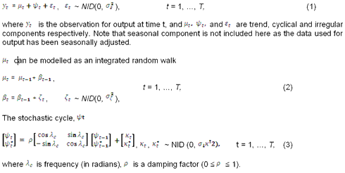
Figure 1: Output and its decomposition into fixed level, stochastic slope, cycle, and irregular.

Using STAMP6.02, we can extract the smoothed estimates of the output gap, which are to be used as a measure of output gap, similarly for consumption and investment. While estimating this, I set the level of the output to be fixed, stochastic slope, irregular, and short cycle (order 1). A stochastic slope is chosen because growth of GDP is not assumed to be constant.

The UC model for inflation can bet set up as

The seasonal component, is only included while estimating the model for CPI as the data on GDP Deflator has been seasonally adjusted.

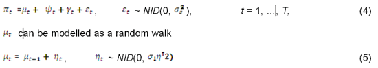
Figure 2: Inflation (CPI) and its decomposition into stochastic level, cycle, seasonal and irregular.

The inflation gap can be obtained in a similar way. Inflation is assumed to be have stochastic level, no slope, seasonal (only for CPI), irregular and short cycle (order 1). As we can see, the erratic movements of inflation in the UK support the trends of other macroeconomic indicators. For example, we can see the rise in inflation in the 1990s recovery.

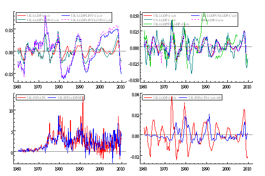
Figure 3: (1) GDP cycle, Bivariate cycles of GDP and investment, Bivariate cycles of GDP and consumption, Trivariate cycles of GDP, investment, and consumption (2) UK GDP cycle, US GDP cycle, France GDP cycle, Bivariate cycle of UK and US GDPs, Bivariate cycles of UK and France GDPs. (3) Inflation measured by CPI and GDP Deflator. (4) Output and inflation gaps (with inflation divided by 100).

As far as Figure 3.1 is concerned, we can see that better estimates of the cycle can be obtained by jointly estimating output with consumption, investment or both (particularly due to larger cyclical movements of investment). Bivariate modelling with the US GDP is done to see if the US GDP cyclical movements affect those of the UK. Considering the fact that Britain’s largest trading partners are the Eurozone countries, I am only going to use the France GDP as there is no complete data for the whole Eurozone excluding the UK. Similarly, I would also do a bivariate modelling of Canadian and the US GDPs.

4. Estimation and Results

4.1 Univariate Model
The unobserved components Phillips curve relating inflation to the output gap can be modelled as

where xt is the output gap, such as the smoothed cycle extracted by running regression (1). Note that instead of contemporaneous output gap, lags of xt can also be used. In this case, β0, β1….., β4 denote the estimated coefficients of the contemporaneous output gap, lags of output gap at one quarter and so on.

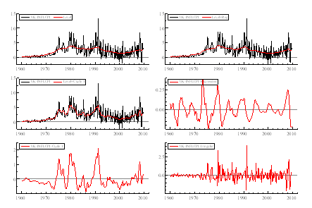
Figure 4: Components (excluding seasonal) in the model relating inflation (CPI) to contemporaneous output gap.

Using the UK data from 1960(1)-2009(4), the estimation of Phillips curve is done using both CPI and GDP deflator. As we can see from the Table 1, the models are mostly significant with lags of the output gap at three and four quarters without any contemporaneous effect, taking into account reasonable Q-statistics (below 24) and values of R2 (not reported in the table). The results do not differ by much even when various bivariate and trivariate cycles are used. The diagnostics are not entirely satisfactory (similar to the results on US data found in Harvey (2008), partially due to the very volatile movements from the 70s to the early 90s – Figure 4.

Estimating the whole sample with GDP Deflator as a measure of inflation seems to provide better results. Referring to Table 2, we can see that there are more significant coefficients on the lags of the output gap at all quarters for all measures of the output gap, although the difference between the results generated with the GDP Deflator and CPI is often relatively small. However, the fact that UK has a very open economy means that CPI should be more relevant as GDP Deflator only measures the level of prices of domestically-produced goods and services while CPI measures average price of all household purchases, which does not exclude imports. Nevertheless, the magnitude of all the significant coefficients seems to be similar to that obtained with CPI.

In fact, if we restrict the sample size from 1995(1)-2009(4), the diagnostics using CPI are greatly improved, particularly for the output gap measured by GDP alone. The contemporaneous output gap provides a relatively good fit, estimating β0 of 43.90 with a t-statistic of 2.30. The estimates of β1 and β2 are 45.40 (2.69238) and 44.28 (2.37) respectively.

Table 1. Measure of Inflation: UK-INFLCPI

Table 2. Measure of Inflation: UK-INFLGDPDEF

Similar results can be seen in the estimation of the Canadian data, although the results tend to be weaker and less significant than the UK – Tables 1a & 2a. Nevertheless, this does not imply the non-existence of the Phillips relation. This could be due to the declining slope of the Phillips curve in the 1980s and 1990s (Beaudry & Doyle, 2003). This can be seen by looking at figure 3a(4) – negative relationship between inflation and output gaps in the early 1990s. The negatively significant figures look particularly worrying when smoothed cycle is extracted from the bivariate model of the US and Canadian GDP since it is expected for the Canadian economy is highly integrated to the US economy, especially since World War II. However, if we start the estimating from 1995(1) using the GDP Deflator, we can get a statistically significant coefficient of the contemporaneous output gap of 91.20, with a t-statistic of 2.14.

4.2 Bivariate Model
Without prior estimation of the output gap, inflation and GDP can be modelled jointly as

The estimation in STAMP6.02 can be done by selecting both measures of inflation and output as two dependent variables and choose the multivariate settings. I have imposed a restriction on irregular by selecting ‘diagonal’ so that the disturbances are assumed to be uncorrelated here. Again, as in the univariate setting, output is chosen to have a fixed level and no seasonal, while inflation is chosen to have no slope. The main result in the estimation is to check the sign and value of β, as it indicates the correlation between the inflation and output gaps. Thus, a positive β means that the Phillips curve relation exists.

Tables 3. UK – Bivariate modelling of Inflation and Output Gap.

The bivariate models estimated over the full period with both CPI and GDP Deflator in the UK work relatively well and make the best use of the data, supporting the results obtained from the univariate modelling. All of the coefficients of β are positive, indicating the relationship between inflation and output gap implied by the Phillips curve. The only concern lies on the difference in the magnitude of β generated by different measures of price index. If we start estimating from 1995, the estimated coefficients grow significantly for both measures – Table 3. Also, if we include the common cycle constraint, the coefficients estimated have the same size with differing order of magnitude, e.g. β = 76.91 when common cycle is imposed on the cycle of CPI.

Table 3a shows the bivariate modelling result for Canada. The results are clearly weaker and less satisfactory than the UK results and there is even a negative coefficient that implies a rejection of the Phillips relation when using CPI. This fact is in line with the declining slope of Canadian Phillips curve in the early 1990s as previously explained in the univariate model. Nevertheless, the correlation still exists if we use GDP Deflator and the values of both are also higher when we restrict the time period.

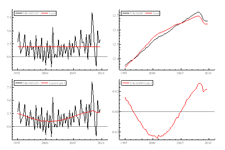
Figure 5: Smoothed components from a bivariate model for GDP and inflation (CPI) (1995-2009).

5. Conclusion
The existence of Phillips curve relation has been widely debatable among macroeconomists around the world. There are also many empirical works devoted to estimate the relation, including Gali and Gertler (1999) and their marginal cost approach, Nason and Smith (2006) on Hybrid NKPC, Lee and Nelson (2007), and so on. Harvey (2008) models the Phillips relation using univariate and bivariate unobserved components.

Harvey (2008) shows that the unobserved components Phillips curve provides a good fit to the US data and the univariate and bivariate models tell the same story. While this might not necessarily be the case in my finding of the UK and Canadian data, there is no reason why the Phillips relation should be rejected here. Various diagrams are included and they show that the extracted components have meaningful interpretation.

Appendix (Diagrams and Tables for Canada)
Figure 1a: Output and its decomposition into fixed level, stochastic slope, cycle, and irregular.

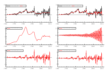
Figure 2a: Inflation (measured by CPI) and its decomposition into stochastic level, cycle, seasonal and irregular.

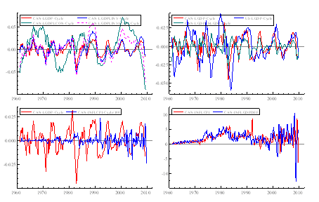
Figure 3a: (1) GDP cycle, Bivariate cycles of GDP and investment, Bivariate cycles of GDP and consumption, Trivariate cycles of GDP, investment, and consumption (2) Canadian GDP cycle, US GDP cycle, Bivariate cycle of Canadian and US GDPs. (3) Inflation measured by CPI and GDP Deflator. (4) Output and inflation gaps (with inflation divided by 100).

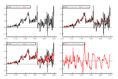
Figure 4a: Components (excluding seasonal) in the model relating inflation (CPI) to contemporaneous output gap.

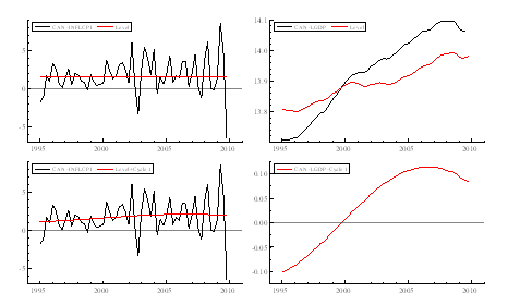
Figure 5a: Smoothed components from a bivariate model for GDP and inflation (GDP Deflator) (1995-2009).

Table 1a. Measure of Inflation: CAN-INFLCPI

Table 2a. Measure of Inflation: CAN-INFLGDPDEF

References
Doyle, Matthew and Beaudry, Paul (2003). What Happened to the Phillips Curve in the 1990s in Canada. Staff General Research Papers 10286, Iowa State University, Department of Economics.

Friedman, Milton (1968). The role of monetary policy. American Economic Review, 58(1), 1-17.

Gali, J. and M. Gertler (1999). Inflation Dynamics: A Structural Econometric Analysis, Journal of Monetary Economics, 44, 195-222.

Harvey, A. C. (1989). Forecasting, Structural Time Series Models and the Kalman Filter. Cambridge: Cambridge University Press.

Harvey, A. C. (2008). Modeling the Phillips Curve with Unobserved Components. CWPE 005.

Harvey, A. C. and T. M. Trimbur (2003). General model-based filters for extracting trends and cycles in economic time series. Review of Economics and Statistics, 85, 244-55.

Harvey, A. C., T. Trimbur and H. van Dijk (2007). Trends and cycles in economic time series: a Bayesian approach. Journal of Econometrics, 140, 618-49.

Koopman, S. J. Harvey, A. C., Doornik J. A. and N. Shephard (2009). STAMP 8.2: Structural Time Series, Analysis, Modeller and Predictor. Timberlake Consultants Ltd., London.

Lee, J. and C. R. Nelson (2007). Expectation horizon and the Phillips curve: the solution to an empirical puzzle. Journal of Applied Econometrics, 22, 161-78.

Mills, Terence (2003). Modelling Trends and Cycles in Economic Time Series. Palgrave Macmillan.

Nason, J.M. and G. W. Smith (2008). Identifying the New Keynesian Phillips curve. Journal of Applied Econometrics, 23(5), 525-551.

Phillips, A. W. (1958). The relation between unemployment and the rate of change of money wages in the United Kingdom, 1861-1957. Economica, 25(100), 283-99.