Research on Forecasting Company Data

Introduction
Forecasts of earnings as predictors of returns is common practice in the investment community and plenty of literature has been written on it discussing and comparing different forecast methods and approaches.

Most commonly, the accuracy of forecasting methods of sell-side professional analysts being compared with the accuracy of time-series models has been a very trending topic in the last few decades as many scholars and analysts keep on trying to find better ways of forecasting earnings to maximise investor’s returns.

In this paper we use the realised earnings per share of the firm Associated British Foods from years 1965 to 2013 and analyse them applying Ordinary Least Squares regression to find out whether the earnings follow a linear trend, quadratic trend or S-shaped curved growth by measuring their errors. We also perform a random walk to forecast the earnings per share from 2014 to 2018 and contrast the results against the best trend model and the actual returns. A forecast using both narrow money supply M0 and broad money supply M3 is also performed and compared with the results of the random walk and the realised returns in order to find out whether time-series models overperform or underperform models that use macroeconomic data and get an idea of what the extent of prediction accuracy of these popular models is. Later, the results will be scrutinised and compared with past research papers.

1. Research on forecasting company data
1.1) The benefits of broadening information set for earnings forecast to include segmental information and leading economic indicators.
As Kinney (1971) reports, one of the main limitations that analysts may encounter when trying to generate accurate company earnings forecasts is holding companies which may own other subsidiary companies or may be operating in more than one industry or sector. The main company may be releasing consolidated reports to try to hide information of other companies that they may own or be an associate of from investors.

When it comes to this kind of companies, analysts may not realise that the numbers that they are taking into consideration may be biased towards one or more of those industries/sectors/subentities and therefore may not be able to predict its future earnings accurately. Earnings from different subentities of the main firm may be somewhat unbalancing the numbers in a way that it would be essentially not possible to predict with accuracy. Did any of the segments contribute more or less than the rest of the entities to the consolidated number?

Kinney reportedly tested the relative predictive power of subentity earnings data for a sample of companies which had voluntarily reported sales and earnings data by subentity to then predict consolidated earnings for years 1968 and 1969.

As he explains in his article, forecasting earnings for a company that operates in pretty much every industry would be relatively easy as getting leading indicators like national gross product would already help massively in determining future numbers. However, when it comes to less diversified companies, taking into consideration GNP alone would not give us a very accurate indication of future performance:

‘On the assumption that such a diversified company would experience earnings growth equal to the rate of growth of GNP, the rate of growth of the economy applied to the earnings of the company should give good predictions of the future earnings of the firm. […] A less diversified firm is diversified in such a way that fluctuations in earnings among divisions offset and […] this rate of growth, of course, [would] be greater or less than the rate of growth for the economy as a whole.’ (Kinney, 1971: 128-129).

He concludes the study by stating that, despite the limitations of his own work (only two reporting periods, a small number of firms and only three segment earnings reports got opinions from accountants), “predictions made on segment sales and earnings data and industry predictions were on the average more accurate than predictions based on models using consolidated performance.” (p. 136).

This would indicate that broadening information set for earnings forecast to include segmental information is usually good for making forecasts of company earnings because it can contribute to the projection of more accurate predictions. As a matter of fact, in the USA, the FASB (Financial Accounting Standard Board) made it mandatory for companies to include segmental financial reporting by releasing the Statement of Financial Accounting Standards -14 (SFAS 14). They felt that by providing segmental information in the early financials, the users of this information – particularly financial analysts – would be able to predict the future earnings of the company with relative ease.

Another factor that seems to contribute positively to better earnings forecasts is the use of leading economic indicators in the models. Chant (1980) and Hussein (1998) wrote articles in which they discussed the benefits of adding information from leading economic indicators in forecast models.

Many reports commenting on forecasts of EPS have relied heavily on extrapolatory models. However, the major problem that lies on these models is the reliability of previous data. To overcome this shortcoming, many scholars have recommended the use of leading economic indicators as a way of forecasting the earnings of a company.

As Chant explains, due to the nature of time-series models of predicting earnings by spotting patterns in a sequence of past numbers, including information from leading indicators can be more useful because they can predict future economic conditions – something that extrapolatory models cannot do on their own. “Generally, lead-indicators are selected for their ability to predict future economic conditions rather than for their time series properties.” (Chant, 1980: 14).

In order to get actual data that could reflect what has been explained above, he got a sample of 218 firms and used several models to forecast one-year-ahead earnings per share, those models being two time-series models (exponential smoothing and average growth) and three others based on leading indicators (money supply M1, stock index and bank loan). It turned out that the money supply M1 model in particular was by far more accurate than any of the other models he had used. Not only did it produce the best results but also the smallest errors, suggesting that monetary aggregates have predictive power.

Also, Hussain made a similar test to see how this would prove beneficial when applied to UK companies, despite of important differences between the US and the UK when it comes to companies’ earnings releases. In order to take Chant’s test further, Hussain tried to find out whether changes in lead times of leading indicators could improve the forecasting models when applied to a wider number of companies from the London stock exchange with no specific requirement on year-end date (Chant’s study focused on companies which year-end was December 31st).

Hussein’s results are similar to those of Chant. In both studies, money supply models (Chant’s M1 and Hussein’s M4) are the ones that produced the most accurate results with the smallest mean and median errors, reaffirming the money aggregate’s predictive properties and its superiority over simple extrapolatory models (when it comes to both mean errors and pair-wise statistical tests).

‘Changes in broad money contain incremental predictive information, relative to similar changes in an individual firm’s earnings over the same time period. This result is consistent with Chant, who finds that the money supply model outperforms models which utilise past earnings data (average-growth and exponential-smoothing models).’ (Hussein, 1998: 278).

According to the literature examined, both including segmental data and adding information from leading indicators in a forecast system can indeed be very useful to produce accurate, fairly reliable predictions that can be used to effectively improve returns on investments.

1.2) Comparing model-based forecasts with those of professional analysts.
The main difference between model-based forecasts and the forecasts produced by analysts would be both the type and amount of information used to produce those predictions.

Model-based systems usually take past numbers and project a future sequence using historical numbers as reference. Adjustments can be applied to these models, as it has been commented on the previous section, by adding information from leading indicators in order to improve their accuracy. However, model-based forecasts usually focus on past performance and it is all processed using technical analysis, which in theory would be an important limitation.

Professional analysts have access to a much wider amount of information that they can use to (presumably) come up with more accurate and useful forecasts. The use of fundamental analysis would make analysts take into consideration things like the time of earnings releases, information from detailed financial reports, future company strategies, company size and many other factors that would prove difficult to blend on a model-based forecast. This could make a big difference on the projection of future income and is the reason why it has always been thought that analysts’ forecasts are generally better than error-measuring focused time-series models (it is why people and firms keep on buying them).

‘Univariate time series forecasts neglect potentially useful information in other time series and therefore do not generally provide the most accurate possible forecasts. Since security analysts process substantially more data than the time series of past earnings, their earnings forecasts should be superior to time series forecasts and provide better measures of market earnings expectations.’ (Brown and Rozeff, 1978: 1).

As an example of what could be thought to be superiority of analysts’ performance, we could have a look at Atiase’s work, who argued that “the degree of unexpected security price changes in response to earnings reports is inversely related to the capitalized value (size) of firms,” (Atiase, 1985: 22) which means that the timing of the release of earnings reports is a key element that moves share prices (mostly when it comes to medium small sized firms).

Another example would be Bamber and her study on trading volume around earnings releases. “Both magnitude of unexpected earnings and firm size were associated with the information content of annual earnings announcements.” (Bamber, 1986: 54). This changes in volume could obviously be used as a tool to place positions with derivatives or buy shares at particular point in time in order to maximise returns.

The questions here would be… how could anyone expect a time-series model take into consideration the timing of an earnings release and the spike that it may cause in a company’s share price? How could it predict the level of volume traded before or after the announcement? How could it apply numbers related to the release of a piece of information that may make the share price of a small firm to skyrocket (or the opposite)? How do we use a variable related to firm size?

Surely, the realised earnings and volume numbers could be used as variables in a model-based forecast to predict future performance, but how useful would it be? Even making the effort of measuring the errors that come out of the model, how could one expect the type of information release that makes those shares to go up and down at a particular point in time to be released again and at regular intervals and causing the same price spikes? A model-based forecast would not be able to do such a thing, no matter the numbers and variables used.

This is perhaps the reason why analysts’ forecasts have been found to be more accurate for short-term predictions (less than 12 months) and naïve models have been found to be more accurate when forecasting long-term numbers (over 12 months) (Paz, 1989).

It can be easily seen that when it comes to short-term projections, the timing of earnings releases, reports and information from balance sheets (fundamental analysis) is key information that investors need to take into consideration in order to make the best out of the movements of the market. This is why “Evidence of significant analyst superiority only exists at shorter horizons.” (Hussein, 1998: 279).

When it comes to predictions longer than 12 months, even if we used past numbers that measure the amount of unexpected earnings obtained from previous spikes in share prices caused by earnings releases (or any other type of information release), the information in a time-series model would be diluted in such a way that it would end up being irrelevant. This could explain why, especially when it comes to small firms, analysts’ superiority on long-term forecasts is not as superior as one would imagine it to be.

1.3) The level of importance of measuring accuracy.
‘Accurate measurement of earnings expectations is essential for studies of firm valuation, cost of capital and the relationship between unanticipated earnings and stock price changes’ (Brown and Rozeff, 1978: 1).

At first sight, the point that the quotation above is making seems unquestionable. It would be obvious to think that in order to obtain the best results on a forecast, one would need to constantly evaluate and measure the accuracy of the models used to know how reliable they are. Therefore, measuring errors and comparing results across models using different variables would seem to be the reasonable thing to do. However, is it really that important to measure accuracy?

Here is a fact. In the past four decades, many studies have been done and many articles have been published about earnings forecasting. The trajectory of these articles, though, is quite peculiar. We could start reading articles from the 1970s which conclude that analysts’ forecasts are overall more accurate than time-series models, then one would read a few articles that state that all market earnings follow random walk models. Later, we find out that not all earnings follow random walk models. Later on, the accuracy of models differs depending on industry and business operations of the firm (Hutira, 2016) and other factors. And it goes on and on.

Forecast accuracy depends on an incredibly wide pool of factors and determinants of accuracy keep on changing along with the economy and the times. This means that regardless of how compelled one may be to find the most accurate forecasting model, its level of accuracy will keep on changing over time.

At the end of the day, what investors need to know is when the market is going to move and what direction it is going to move to so they can take appropriate decisions. This can be forecasted by looking at leading indicators and using models that have been proven to give results similar to realised results.

When we are forecasting earnings, we are trying to find out what will happen in the future. Nobody can know exactly what will happen in the future. Trying to get very high levels of accuracy may as well be a lost battle – unless one understands that accuracy measuring must be used as a flexible tool rather than a fixed, ever-constant benchmark.

2. Analysing the data
In this section, we will estimate the ability of the linear trend model, the quadratic model and the s-shaped model in analysing the relationship between the EPS of the company Associated British Foods plc. (the dependent variable) and the time counter (the independent variable) by using the actual data from 1965 to 2013.

After the estimations, the model which provides the best fit to the data will be highlighted. We will also predict the EPS of the company from years 2014-2018 based on those three models. The mean absolute error will also be calculated, and the models will be ranked from the best (the model which has the lowest mean absolute error) to the worst (the model which has the highest mean absolute error).

Finally, a random walk and two money supply models will be employed to forecast the EPS of the company from 2014-2018. The resulting forecast will be compared with the results of the best model with the lowest mean absolute error.

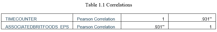
Before we start estimating the models, correlation analysis will be used to find out if there is a significant relationship between the target variables. The following table shows that the Associated British Food’s EPS is strongly related to the Time Counter variable, with 0.931 of Pearson Correlation. Therefore, the analysis of the true relationship between the two variables is necessary and those three OLS regression-based models mentioned above will be performed to analyse the relationship between these two variables.

By applying the data on SPSS, we get graphical patterns of these three different OLS regression-based models (the linear trend model, the quadratic model and the s-shaped model).

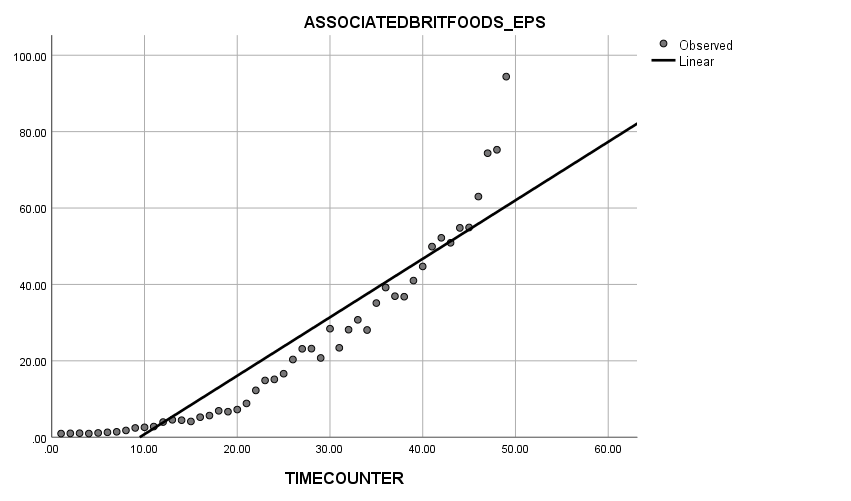
Firstly, the linear trend model presents a straight line with an increasing trend with a relatively large amount of actual figures around the line from Time counter of 10 to nearly 45. However, after the time counter of 45, the EPS of the company show a sudden rise which deviates from the straight line dramatically.

Graph 1.1 Linear Trend

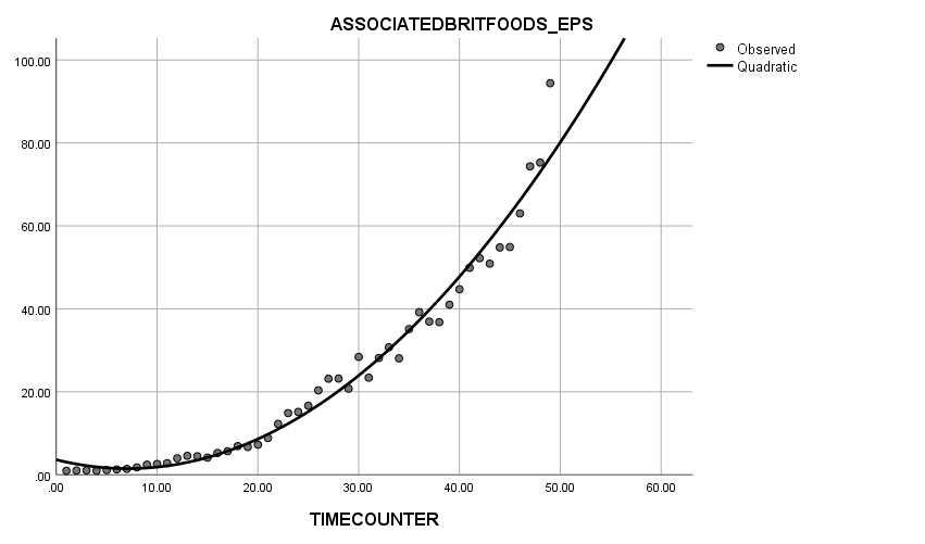
Secondly, when looking at the quadratic trend model, it is quite obvious that almost all the actual figures were distributed around the curve except for a few observations. The curve fits the actual figure relatively well.

Graph 1.2 Quadratic Trend

Thirdly, when it comes to the s-shape curve, a huge difference between the growth trend of the actual figures and the curve pattern can be easily observed: most of the actual data did not match with the curve. The slope of the actual data is clearly different from the slope of the curve of the model.

Graph 1.3 S-shape Curve

Conclusively, by looking at these three patterns above, perhaps it could be argued that the quadratic trend is most likely to have the least standard deviation of all these three models, which indicates that the quadratic model may be the best model for the given data, as it shows the best fit.

Additionally, the R square figure can also help to identify the best model. The R square figures of the three models are as shown below:

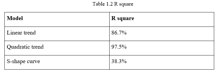
According to the table above, the linear trend model has a relatively high R square of 86.7% while the R square of the quadratic trend model is 97.5%. However, the R square of the s-shaped curve model is merely 38.3%. These figures mean that in the quadratic model, 97.5% of the variation in the dependent variable can be explained by the independent variable, which is the highest of the three models. Therefore, the quadratic model is potentially the best fit based on the analysis of the R square figures.

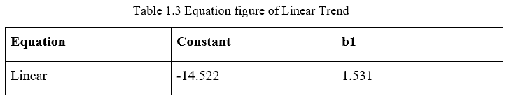
Moreover, by adopting the relevant figures from the curve estimation table, equations for those three models can be established in order to forecast the EPS of Associated British Foods from year 2014 to year 2018.

Firstly, the equation of the linear trend model can be shown as: Yt = b1 + b2.t, where Yt is EPS, b1 is the constant, b2 is the b1 in the estimation table and t is the time counter, then we can get the final equation: EPS=-14.522+1.531t.

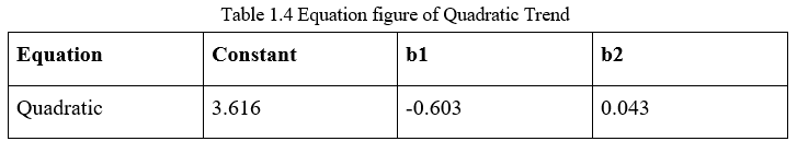
Secondly, the equation of the quadratic trend model is as follows: Yt = b1 + b2t + b3t², where Yt is EPS, b1 is the constant, b2 is the b1 in the table, b3 is the b2 in the table and t is the time counter. Then the equation can be written as EPS=3.616+(-0.603t)+0.043t².

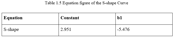
Finally, the equation of the s-shape curve is presented as: Yt = e^{k + (h/t)}, where k > 0 and h < 0, Yt is EPS, k is the constant, h is the b1 in the table, and t is the time counter, therefore the final equation could be shown as EPS=e^{2.951+(-5.476/t)}.

By applying these three equations above, forecasts for the company’s EPS from 2014 to 2018 can be calculated and be compared with the actual data we have. The calculations and comparisons are presented in the table below:

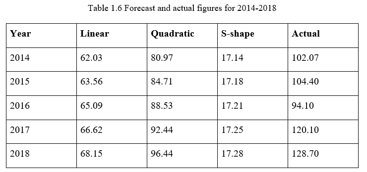
Based on the table above, it could be argued that the quadratic model shows the closest results to the actual data, while the s-shaped model shows a very inaccurate forecast.

Nevertheless, another important factor to measure the effectiveness of the models is the trend of the forecasting data, since it can tell us whether the model can be considered to be a reliable tool for forecasting future data or not. According to the table above, the EPS predicted by the quadratic model shows a significant increasing trend during the 5-year period with the growth of approximately 0.4 pence per year which could be regarded as the best trend fit compared with the overall trend of the actual data. However, in terms of both accuracy and trend, the other two models have shown relatively poor performances compared with the quadratic model.

Another approach can be used to check the accuracy of the models; calculating the mean absolute error. By calculating the mean absolute error of the models, we can rank the model from the best (shows the lowest errors) to the worst (shows the highest errors). The formula of the mean absolute error is given as: MAE=Ʃni=1|Yi-Xi|/n, where Yi is the estimated EPS and Xi is the actual EPS. Thus, a mean absolute error table was drawn and shown below:

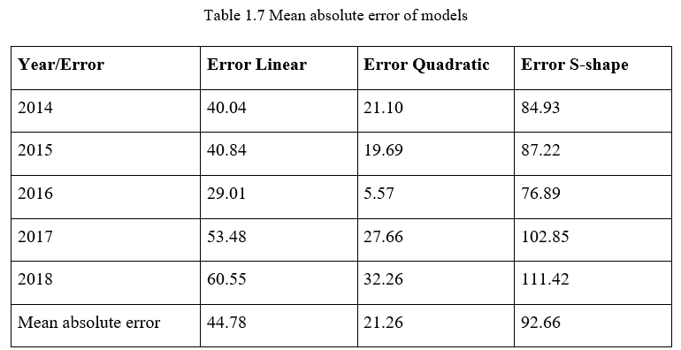
According to this table, we can probably say that the quadratic model has the lowest errors (much lower than the errors made by the other two models) while the s-shaped model made the highest errors. Therefore, the ranking of models from the best to the worst can be shown as Quadratic>Linear>S-shape.

What is left to do now is to compare the forecast of the best model above (the quadratic model), the random walk model and the two money supply models for the period 2014-2018.

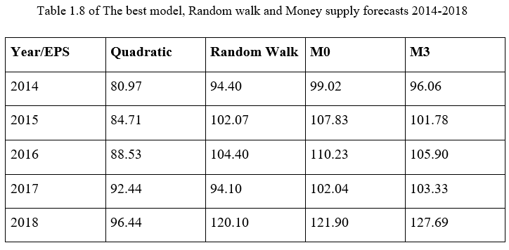
According to the tables above, it seems that the quadratic model predicted the lowest EPS for the company from 2014-2018 compared to the ones predicted by the random walk and the two money supply models. However, the money supply models (both M0 and M3) predicted the highest EPS numbers in general. The overall EPS predicted by the random walk model were somewhere between the EPS numbers predicted by the quadratic model and the ones predicted by the money supply models.

Looking at the following table, we could say that the quadratic model made more errors than the random walk model and the money supply models in predicting the company’s EPS, except for the EPS for 2016 (the EPS for 2016 predicted by the quadratic model actually has the smallest error among the four models).

Table 1.9 Mean absolute error of the best model, Random walk and Money supply

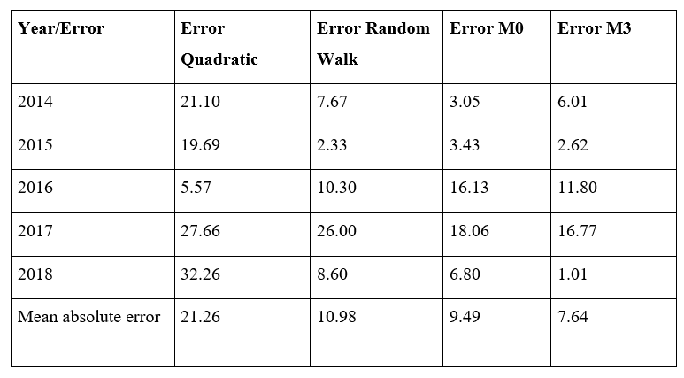
Accordingly, although the trend of growth of the EPS predicted by the quadratic model is quite consistent with the actual trend as has been outlined above, the quadratic model should be regarded as the most inaccurate model of these four models as a whole. Nevertheless, in general, the M3 money supply model predicted the EPS of the company with the lowest errors compared to quadratic model, random walk and M0 money supply model. Therefore, based on the existing data, it could be argued that the M3 money supply model made the most accurate forecast among these four models in terms of the EPS for the company from 2014 to 2018 while the quadratic model gave us the poorest overall predictions compared with the other three models.

3. Discussion.

3.1) Comparing the performance of the models to the random walk – Explanation of results.
The results of the linear trend model and S-shaped model are not very good in comparison to the random walk. However, the result of the quadratic trend and money supply models (both M0 and M3) accurately forecasted the company’s earnings per share. The tables and graphs above show that both the linear trend and the S-shaped models have higher mean absolute errors than the quadratic trend model and the random walk.

The results obtained by the Linear trend and S-shaped trend models are very different from the actual historical figures from 1965 to 2013. The linear trend model presents a straight line, but the firm’s earnings per share did not comply with a linear growth trend. Therefore, this model makes an incorrect prediction of the latter figures of Associated British Foods’ earnings. Also, there seems to be a huge difference between the results of the S-shaped trend model and the actual data. In a nutshell, the two models don’t get even close to being accurate predictive models of earnings in this firm.

However, when comparing the latter two models with the quadratic trend model, one could very easily see the difference in performance. The quadratic trend model performed really well. This model matched almost all the past numbers and forecasted the future tendency of the firm’s earnings per share.

Looking at the random walk, it has a clear advantage over all the trend models. Comparing the trend models with the random walk, the latter performed much better as it produced the lowest error ranking. Not bad at all for a time-series model and low-cost alternative of making predictions.

We must also note that even though the quadratic trend model was found to match the growth trend of the company accurately and the random walk produced fairly accurate predictions, regardless of these good results, there is one big champion in this project – the money supply models, in particular the broad money supply M3 one. Not only did this model produced the most accurate earnings-per-share numbers, but also made the lowest errors of all the models used, as it has been shown on the tables.
The difference in performance between all these models would be explained as follows.

Firstly, model-based systems usually use historical figures to predict the future trend, but they do not consider the changes that may take place in the future. The linear trend, quadratic trend and S-shaped trend models use old figures of the Associated British Foods’ earnings from 1965 to 2013. These models are built with historical data and the model’s own formula to try and find the growth tendency and also forecast the firm’s EPS from 2014 to 2018.

In relation to the earnings forecast of Associated British Foods, we concluded that out of the three OLS-based regression models, the quadratic trend model was the best suited model in terms of error ranking. Because of the fact that these models focus only on the past performance of the company, these three models ignore the influence of changes in the share price. EPS are affected not only by internal factors but also external factors. Changes in macroeconomic factors and in the whole industry will almost definitely influence the company’s earnings.

Therefore, when calculating future numbers, it is logical to use variables that reflect those changes in macroeconomic factors as this could theoretically make the forecasting model to yield more accurate results. This is the reason why the money supply information is added to the forecasting formula and the reason why the money supply models in this project present the most accurate results with the tiniest errors.

It would also be wise to stand out that, although the figures obtained from the money supply models are better than the ones from the trend models, the results are still different to the realised numbers. This may be because quarterly earnings are usually not disclosed in the UK.

When making predictions, it is important to use figures that do not delay the real operating activities too much as this could reduce the predictive quality of the model. Using quarterly earnings or semi-annual earnings numbers instead of annual numbers would probably improve accuracy.

Still, the money supply model remains the winner as the macroeconomic information within it makes the model to yield the best results when compared with any of the other models employed in this project.

It is worth mentioning that the random walk also performed much better that the trend models but at the same time was outperformed by both money supply models. The explanation for this phenomenon would be found in the actual gears of the devices; the random walk uses the data from the previous year to forecast the present year’s earnings. On the other hand, as it has been already mentioned, the money supply models reflect changes that occurred in the economy with a time lag of 12 months, which allows it to produce much more accurate forecasts. These results confirm the findings of Chant and Hussein, who came to the same conclusions.

Chant compared the naïve model (Random walk) with Money supply, Bank loan and stock index models along with three time-series models. In his findings, he had observed that the Money supply model was the most consistent model with predictions close to the actuals. Also, in ranking the models based on errors, Chant observed that the Money supply model dominated by the other models with the lowest error rankings.

Hussein went one step ahead and compared the Random walk model with the narrow and broad money supply models and random walk with drift model wherein the same mirrored the Money Supply model. It is imperative to note that the Money supply model considers the changes in the Macroeconomic factors whereas the RWD model considers the changes that happened within the firm. However, when the tests were conducted to test the accuracy of the data that were predicted, Hussain too came to the conclusion that the money supply model performed much better in comparison to all the other models and that the results achieved were also similar to those of Chant.

3.2 Limitations of the models when being used on other companies.
While making earnings forecast analysis for other firms, due care must be taken. Using the M3 money supply model for other firms of comparable size to Associated British foods may yield good results, but for other firms that are not of comparable size, the same may not yield the best results.

One needs to be very careful when selecting adequate prediction models to make an analysis of earnings per share. Using the M3 money supply on a firm/company which is operating in a cashless environment may not yield the best results in predicting the EPS.

For example, companies that deal with manufacturing of industrial products like industrial chemicals, using the money supply model will probably not produce the best forecast. Also, for a start-up firm which is in the process of raising initial funds and significant operations have not begun, predicting their earnings with the help of the money supply model may not yield the best of results either.

Therefore, while selecting the earnings forecast model for a firm or a company, we need to ensure that, based on the size of the firm and type of industry in which the company operates, the most appropriate model is chosen. We must keep this in mind in order to make sure that the earnings forecast model is adequately using the relevant data and information in order to make the most accurate forecast possible. Not always the broad money supply model will be adequate for all of firms due to the huge money flow involved in such model.

Since 2006, the M3 model is not included in the periodical reporting of the Federal Reserve. This is because the additional liquid components of the M3 model did not appear to convey more economic information that was already being captured by the M2 model. Therefore, for any firm or a company which is operating out of the US or whose operations are mainly concentrated in the US, the use of the M3 model may not be the best at predicting the earnings of a company.

It is noticed that diversity of payment method leads to an obvious decrease of the use of cash and some countries are even planning on researching and developing digital currencies based on new technology such as blockchain. Therefore, in an era of cashless transactions and digital currency, we must remember that the level of relevance of the money supply model in predicting the earnings of a company could fluctuate. In countries like Sweden during the year 2016, it was reported that only 2% of the value was cash transactions and only 20% of the total retail transactions were done by cash. If we go by these trends, soon enough the whole flow of money in the economy will be practically non-existent. We must start developing new scientific models to predict the flow of earnings of companies which value cannot be influenced by the money supply indicator.