Effects of toxic waste on Grasmere aquatic ecosystem
Abstract
Ecosystems can become unbalanced through pollutant effects, and their stability becomes disturbed. This investigation is concerned with the effects of toxicants on humans and wildlife in the Grasmere aquatic ecosystem. In this report, ecological risk assessments are carried out and a mathematical model is developed.
The continuously stirred tank reactor (CSTR) was chosen for the reaction scheme because it minimises the many steps involved in solving steady state conservative systems. The model considers four separate lakes: Grasmere, Rydal Water and Windermere (split into two). The findings of this study suggest that it is impossible to assess all of the species in the ecosystem because they vary in their susceptibility to copper contamination. Representative species were chosen for each trophic level based on several criteria.
The scope of this investigation is limited to developing a preliminary mathematical model. Future work will refine the model and compare the results obtained with previous studies.
Statement of problem
This report investigates the effects of toxicants on humans and wildlife in an aquatic ecosystem. The chemical stressor in this investigation is toxic waste from industrial processes. The study site is set in Grasmere in the English Lake District. The contaminant source is dissolved copper; it is supposed that due to mining operations, a continuous release of 40,000 kg of dissolved copper is initiated.
Objectives
The objectives of the current paper were:
- To review the published literature on the water quality and catchment of Grasmere Lake in the English Lake District
- To assess the severity of potential releases of toxic material for the aquatic ecosystems
- To analyse the possible pathways between toxic material and receptors using a conceptual model and food chain analysis
- To develop a preliminary conceptual model and convert it to a mathematical model.
Study site
Before formulating a conceptual model, the physical boundaries of the region were defined. Grasmere is one of the smaller of the main lakes of the English Lake District; it is set in a valley that is surrounded by hills. We limit our analysis to a small region. Within these limitations, we see the flow as originating in the north-west from Grasmere to the output at Newby Bridge at the south end. It can be seen from Figure 2A that run-off from the hills runs down through several rivers and major lakes. Therefore, the following water bodies will be impacted by heavy-metal pollution release in Grasmere:
- Grasmere
- Rydal Water
- River Rothay: flows between Grasmere and Rydal Water
- River Brathay: the River Rothay joins the River Brathay at Ambleside, from where they flow on to pour their combined waters into the northern end of Lake Windermere
- Windermere: the largest (14.8 km²) natural lake in England. It comprises a north basin (area 8.1 km², depth 64m) and a south basin
Figure 1: Map of Grasmere showing the catchment boundary and the major inflow and outflow streams
Source: Bennion H., Appleby P. G., Boyle J. J., Carvalho L., Luckes S. J., and Henderson A. C. G. (2000). Water quality investigation of Loweswater, Cumbria. Final Report to the Environment Agency. Environmental Change Research Centre.
In this report, Chapter 1 has outlined the problem with mining waste and defined the study site. Existing data are reviewed in Chapter 2 to identify populations and ecosystems at risk. The possible pathways are considered to generate a preliminary conceptual model. Understanding how these systems respond to stressors will provide a basis for well-informed decisions for the selection of receptors and end points in Chapter 3. A mathematical model will be developed in Chapter 4. Choices will be justified based on estimates of the exposure concentration for each population.
Conceptual model
This section seeks to implement risk assessments to build a conceptual model for analysing the effects of toxicants on humans and wildlife on the site. The reasons for developing the model are that it shows all of the sources, receptors, and transport and exposure pathways for the system.
Exposure analysis
The contaminant source is dissolved copper; it is supposed that due to mining operations, a continuous release of dissolved copper is initiated. Particularly important are exposure concentration and frequency of release. The loading is 40 tons (40,000 kg) per day. This may lead to contamination of drinking water supplies.
A conceptual diagram was constructed to represent this (see Figure 2). According to the conceptual model developed, contaminants enter the system from a point source, here it is wastewater discharged into a river. The dissolved copper is transported through interactions with sediment and water. Several secondary release mechanisms then transport the contaminants through the systems. These are plant uptake, percolation and sorption/desorption.
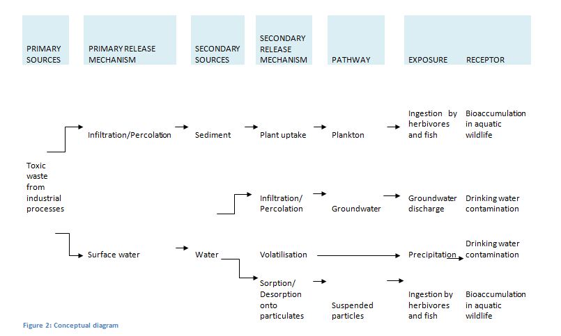
Figure 2: Conceptual Diagram
Additional data needs for conceptual model
Modelling of discharge
The conceptual model highlighted all of the exposure pathways and receptors that are of interest. It was clear that additional data and simplification were needed to support the conversion of the conceptual model to a mathematical model. ne of the exposure pathways concerned the absorption and desorption of copper contaminants into the water. It can be seen from Figure 2 that this pathway results in suspended particles which are ingested by aquatic wildlife. It should also be noted that only the ionic form of copper is toxic. To model the partition of copper in ionic form would have been very complicated. To simplify, the discharge was modelled as a continuous release of dissolved copper ions.
Additionally, information necessary to determine the mixing of the copper ions was difficult to obtain. The usual approach for this type of problem is to utilise a model of the lake as a steady state (time invariant) conservative system using CSTRs. This assumes the complete mixing of the pollutant in the water. This was considered to be the most suitable approach because it involves simple algebraic equations and mathematically it is not very complex.
Selection of receptors
One problem area that required more data was copper uptake by plants. Aquatic organisms may accumulate copper to high levels in their tissues by bioaccumulation. It was noted that Windermere is currently home to a range of plant communities. The wildlife in the Windermere catchment area also comprises approximately 16 species. Of these, nine are minor species (such as insects, Crustacea and Mollusca). To study the effects of toxicants on wildlife, seven species could be included as receptors of potential concern. These species have a large biomass of fish per hectare. They are:
Arctic charr (Salvelinus alpinus), Atlantic salmon (Salmo salar), brown trout (Salmo trutta), European eel (Anguilla anguilla), perch (Perca fluviatilis), pike (Esox lucius) and roach (Rutilus rutilus).
A food chain analysis was performed to investigate how the receptors were exposed to bio-accumulated environmental contaminants. This exposure route is illustrated in Figure 3
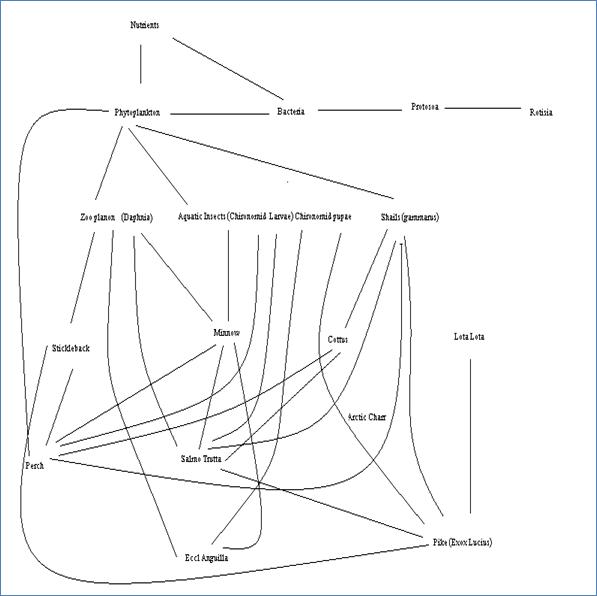
Figure 3 : Food Chain
It was concluded that test organisms should be chosen as representative of each important trophic level. The eel (Anguilla anguilla) was selected as a receptor; eels are the top predators in this ecosystem. They feed on Daphnia, which is a primary consumer of phytoplankton.
Aquatic organisms can accumulate copper to high levels in their tissues by bioaccumulation, which can rise to levels even greater than the external concentration. The estimated total fish biomass was ![]()
![]() and the total eel biomass in the study site was
and the total eel biomass in the study site was![]() . Therefore, it was decided that the potential for bioaccumulation should not be considered in the mathematical model because it is so small.
. Therefore, it was decided that the potential for bioaccumulation should not be considered in the mathematical model because it is so small.
Instead, the analysis would use the external water and sediment concentration as an indicator. In the scenario for the phytoplankton receptor, the model’s objective would be to find the time it will take the sediment to reach its permissible copper concentration based on acute and chronic effects. One of the implications of this approach is that the species are found at different water levels. Windermere is a lake of glacial origin, so the water is stationary near the bottom of the lake.
Flow direction can be constructed by modelling the lake as two layers. In this approach, the top layer flows as normal and the bottom layer is stationary. Figure 4 demonstrates a method for modelling diffusion across a solid boundary and a fluid flow. This can be applied in the proposed model; it is assumed that there is complete mixing in the CSTR in the top layer. Then the copper contaminant moves to and from the layer by diffusion. This is known as Transport Controlled Flux.
Figure 4 : Two phase flow model
It is intuitively obvious that the water close to the surface would be more polluted or have a higher concentration of copper. Thus, species living in this part of the lake would be more exposed to the risk. On the other hand, species living closer to the bottom would not be impacted as much. Concerning the carnivores (eels), hydro-acoustic surveys confirm that the majority of eels are found near the surface. Additionally, no eels were observed at a depth greater than 15m. This information is presented in Figure 5.
Figure 5 : Abundance of eels in Windermere at different depths at low water level and at night
Source: Schulze T., Kahl U., Radke R., and Benndorf, J. (2004). Consumption, abundance and habitat use of Anguilla anguilla in a mesotrophic reservoir. Journal of Fish Biology, 65, 1543–1562
Based on the information found, the lake could potentially be modelled as two layers. Eels can be used as a receptor to monitor the water quality of the flowing fluid layer. For the bottom layer, a bethnic organism such as Daphnia was the most suitable. These are biota that live on, or very near, the bottom of the sea, a river or a lake. A bottom-feeding herbivore could be used as a receptor at high deep water levels. It is also proposed that a third sediment layer is used with a phytoplankton receptor. The next task was to select suitable end points for the model.
Selection of end points
Additional data needs were also identified within the food chain. It was found that the different species of fish vary in their susceptibility to copper contamination. A key issue was to determine a significant end point for the mathematical model. It was mentioned earlier that ecosystems may become unbalanced through pollutant effects as the stability becomes disturbed. The ecological effects fall into two categories:
- Lethal effect – where species are killed
- Sub-lethal effects – where species remain alive but with reduced ability.
This problem was addressed by comparing aqueous toxicity data from toxicity profiles for Windermere. The response of species to copper contamination is usually modelled by assessment of the sub-lethal effects LE50, as illustrated in Figure 4. This is the concentration that brings about sub-lethal effects in 50 per cent of the individuals in the test population.
Figure 6 : Empirical distribution functions for acute toxicity and chronic toxicity of copper to fish and aquatic vertebrates and for individual measurements of copper in sediment pore water (3.02 to 4.04). Vertical lines are acute and chronic water quality criteria
Source: Suter G., Efroymson R., Sample B., and Jones D. (2000). Ecological Risk Assessment for Contaminated Sites. CRC Press.
A key task was to select a significant end point for each receptor. The concentration that 50 per cent of species developed sub-lethal effects
| Trophic level | Representative species | LE50 (mg/L) |
| Plant | Phytoplankton | 0.005 |
| Herbivore | Daphnia | 0.1 |
| Carnivore | Eel | 1.0 |
Table 1: LE50 for representative species in each trophic level
From the literature review, it was found that sources of drinking water to Manchester include rivers, streams and lakes in the study site. It should be noted that its water extraction point is situated somewhere in Windermere. For the sake of brevity, it was decided to omit this feature from the model. It is assumed that the extraction point is at the output of Windermere.
The standard for copper concentration is 0.02 milligrams per litre (mg/L). In this investigation, the end point for humans is when the copper concentration rises above the drinking water standard (0.02 mg/L). This is presented as the vertical line in Figure 5.
To summarise the findings of the chapter:
- Test organisms were chosen as representative of each important trophic level
- The end points were based on the concentration that 50 per cent of the species developed sub-lethal effects
- To simulate the real-life flow of Windermere, a two phase flow needed to be implemented.
Mathematical model description
Modelling objectives
Before proceeding, the modelling objectives and the end use of the model were decided. t should be a basic model, it must be easy to understand, contain few errors and be quick and easy to build, run and analyse. This model will be used:
- To find the time it will take the lake to reach its permissible copper concentration based on end points. These are 0.02 mg/L, 0.01mg/L and 0.1 mg/L
- To find the time it will take the sediment to reach its permissible copper concentration of 0.005 mg/L
- To better understand the parameters that the model depends largely on
- To refine the model to obtain a more accurate estimate.
These objectives determined the required levels of model detail and model accuracy. For this first model, 100 per cent accuracy is not critical. The advantage of performing such a simple model is that it gives quicker results which can be assimilated. We want to gain a better understanding of the factors that influence the entire process and the relationships between the input and the output.
Given these modelling objectives, a number of simplifications were made. Here, the accuracy is sacrificed to reduce the complexity of the model.
Background
To simplify the model, it was broken down into two parts. These are the complete CSTR mixing processes and diffusion processes.
In this model, it is assumed that the pollution is completely mixed in the lake. A set of four CSTRs in series are used to simulate the hydrodynamic processes in the system. The CSTR was chosen for this reaction scheme because it minimises the many steps involved in solving steady state conservative systems. The model considers four separate lakes: Grasmere, Rydal Water and Windermere (split into the north basin and the south basin).
A combination of CSTRs and plug flow reactors (PFRs) was initially considered to simulate the lakes and the rivers that feed them. However, the rivers should be omitted because they have small volumes relative to Grasmere, Rydal Water and Windermere. It was concluded that it would make the analysis more complicated than was necessary to meet the objectives.
The basic description of the scenario is that there is a mining operation that discharges a continuous release of dissolved copper into the lake. One option was to assume that the entire mass of ![]()
![]() of contaminant is quickly dumped into a perfectly-mixed vessel at time
of contaminant is quickly dumped into a perfectly-mixed vessel at time![]() . However, an instantaneous discharge is unrealistic and would not meet all of the objectives.
. However, an instantaneous discharge is unrealistic and would not meet all of the objectives.
There are three objectives in the model; the first is to compute the mean time taken by the CSTR in the Windermere south basin to reach the end point when the copper concentration rises above the drinking water standard (0.02 mg/L) and the time taken by the sediment to reach its maximum permissible level.
To achieve this, 10,000 kg of copper is added to Grasmere averaged over six hours. he model is discrete and only makes calculations every six hours (this is defined as an ‘interval’). Every six hours a new concentration is calculated for each lake. The total mass of copper that enters the lake is calculated from the initial loading (Grasmere) or what has left the previous lake in the last six hours. he focus of the model is to define a mass budget of copper for each lake based on the input and output of polluted water.
Model 1: Modelling of lakes as a CSTR
This section describes the first methodology for the modelling of the migration of pollution through the lakes of the system.
Modelling lakes
Modelling individual lakes as CSTRs allows for a simplified balance of input and output concentrations to be assumed. As large volumes of water are moved within the lakes at high flow rates, it can be assumed that the lakes are well-mixed. This assumption underlies the validity of the model. The interconnecting rivers have a much smaller volume than that of the lakes. The direct participation of the rivers within the model has therefore been omitted. Instead, flow from one lake to another has been assumed to be delayed by a short time equivalent to the time taken for the volume of water contained by a river to be fully exchanged. Otherwise the flow of water between the lakes has been treated by a series of CSTRs.
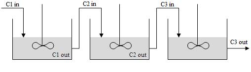
Figure 7: Lakes are presented by a series of CSTRs with the output of one lake providing the input for the next
An expression for the accumulation of a particular chemical species within a CSTR can be deduced by its mass balance. For a CSTR, it is observed that the output mass is the mass leaving the current lake to go into the next lake. The difference between these is what has accumulated in the lake, and this determines the lake concentration. Calculations start with the observation of the following relationship:
![]()
![]()
Equation 1
This is summarised in the equation
![]()
![]()
Equation 2
where ![]()
![]() is influent concentration [ML-3],
is influent concentration [ML-3], ![]() is effluent concentration [ML-3],
is effluent concentration [ML-3], ![]() is reaction rate [ML-3 T-1] and
is reaction rate [ML-3 T-1] and ![]() is the volume of the tank reactor. The equation can be simplified for the time-dependent output concentration
is the volume of the tank reactor. The equation can be simplified for the time-dependent output concentration ![]() as follows:
as follows:
![]()
![]()
Equation 3
The residual time ![]()
![]() represents the time taken to fully replace the volume of the system through the movement of the fluid. It is given by
represents the time taken to fully replace the volume of the system through the movement of the fluid. It is given by
![]()
![]()
Equation 4
Equation 5
Equation 6
Integrating Equation 6 yields the following equation with a constant resulting from indefinite integration:
Equation 7
At the start time for the model the concentration of the lake is at ambient levels of copper before pollution input into Grasmere. The concentration of the lake is therefore C = C0 at t = 0 for an ambient copper concentration C0:
Equation 8
The expression for K (Equation 8) can be substituted into Equation 7 to give a time-dependent equation for concentration:
Equation 9
Equation 10
Equation 11
The ambient concentration of copper independent of pollution is assumed to be negligible and constant. With this assumption, the equation can be simplified:
Equation 12
From Equation 10, it can be seen that the output concentration of the lake tends to the input concentration as t > φ. As the loading of copper increases in the lake, the concentration throughout the volume of water becomes equivalent to the input concentration. For this condition, the lake has reached equilibrium, with input and output concentrations equal. If the rate of outflow is not greater than the rate of inflow, then accumulation due to influence should not increase beyond input concentration.
To achieve the objectives of the model, it was decided to reject the two phase flow model. This is because there are many steps involved in the calculations, so this would add to the complexity of the model. Most importantly, it is required that the model should have as few free parameters as possible. However, the transport reaction model depends on a number of factors, including the surface area, the diffusion coefficient and depth of layer. As a result, it would take substantially longer to run the model, and the uncertainty of the model increases.
Conclusion
From the preliminary results, it can be safely concluded that the CSTR model is quite accurate for analysing the effects of toxicants on humans and wildlife on the site. A combination of CSTRs and PFRs was rejected because it would make the analysis more complicated than was necessary to meet the objectives.
The scope of this investigation is limited to developing a preliminary mathematical model. The next reports will present the results and discuss the findings and recommendations.
Bibliography
- Alex J., Risholt L. P., and Schilling W. (1999). Integrated modeling system for simulation and optimization of wastewater systems. Eighth International Conference on Urban Storm Drainage. Sydney, Australia. 30 August–3 September 1999, 1553–1561.
- Bennion H., Appleby P. G., Boyle J. J., Carvalho L., Luckes S. J., and Henderson A. C. G. (2000). Water quality investigation of Loweswater, Cumbria. Final Report to the Environment Agency. Environmental Change Research Centre.
- Garsdal H., Mark O., Dorge J. and Jepsen S-E. (1995). Mousetrap: modelling of water quality processes and the interaction of sediments and pollutants in sewers. Wat. Sci. Tech., 31 (7), 373–380.
- Rauch W., Henze M., Koncsos L., Reichert P., Shanahan P., Somlyódy L., and Vanrolleghem P. (1998b). River Water Quality Modeling: I. State of the Art. Wat. Sci. Tech., 38 (11), 237–244.
- Schulze T., Kahl U., Radke R., and Benndorf J. (2004). Consumption, abundance and habitat use of Anguilla anguilla in a mesotrophic reservoir. Journal of Fish Biology, 65, 1543–1562.
- Suter G., Efroymson R., Sample B., and Jones D. (2000). Ecological Risk Assessment for Contaminated Sites. CRC Press.