The relationship between inflation and economic growth (GDP): an empirical analysis
1) Introduction
For many years the relationship between economic growth and inflation has been one of the most widely researched topics in macroeconomics. In economics, inflation is defined as the increase in the level of prices and economic growth and is usually defined as the Gross Domestic Product (GDP). It measures the market values of a country’s final goods in a specified period: GDP = Consumption + Investment + Government Expenditure + Net Exports (Exports – Imports).
An increase in inflation means that prices have risen. With an increase in inflation, there is a decline in the purchasing power of money, which reduces consumption and therefore GDP decreases. High inflation can make investments less desirable, since it creates uncertainty for the future and it can also affect the balance of payments because exports become more expensive. As a result, GDP is decreases further. So it appears that GDP is negatively related to inflation. However, there are studies indicating that there may also be a positive relationship. The Phillips curve, for example, shows that high inflation is consistent with low rates of unemployment, implying that there is a positive impact on economic growth.
In this paper I examine empirically the relationship between inflation and economic growth (GDP) in the United Kingdom. The paper is organised as follows: section 2 gives the literature review; section 3 describes the data; section 4 shows the methodology and the empirical evidence; and section 5 provides the summary of the study and conclusions reached.
2) Literature review
Various studies have been presented on the issue of inflation and economic growth. Some of them are briefly discussed here.
Fischer (1993) showed that inflation and growth are negatively related. More specifically, he argues that growth, investments and productivity are negatively related to inflation and that capital accumulation and productivity growth are also negatively affected by budget deficits. Moreover, he states that some exceptional cases show that even though high growth is not necessarily associated with low inflation and small budget deficits, high rates of inflation are not consistent with permanent growth.
Barro (1995) examined data for almost 100 countries for the period between 1960 and 1990 and found that the impact of inflation on growth and investment is significantly negative, given that a number of countries characteristics are constant. An average increase in inflation of ten per cent leads to a decrease of GDP and investment by 0.2 to 0.3 and 0.4 to 0.6 respectively. He also showed that even if inflation has a small impact on growth, this appears to be significant in the long run.
Bruno and Easterly (1996) examined the relationship between inflation and economic growth and they found that this relationship exists only if there are high inflation rates. To determine the high rates of inflation, they set a threshold of 40 per cent. Above this threshold, inflation has a temporally negative impact on growth, whereas below this threshold, they found no robust relationship. The decrease in growth is temporary because after a high inflation crisis, the economy quickly recovers to its previous level. During this recovery, the economy can regain most, if not all of the loss of the economy’s output. Their results are robust after controlling for other factors such as external shocks.
Ghosh and Phillips (1998) studied the relationship between inflation and GDP for a large set of IMF countries for the period from 1960 to 1996. They found that, generally, the coefficient, with respect to inflation, was negative. The findings were statistically significant. More specifically, they found two nonlinearities in the inflation− growth relationship. The relationship between these appeared to be negative for very low inflation rates (around two to three per cent). They also found a negative correlation for higher values but the relationship was convex, meaning that a decline in growth related to an increase of from ten to 20 per cent inflation was larger than that related to an increase in inflation of from 40 to 50 per cent.
3) The data
We used quarterly time series data from the Office for National Statistics United Kingdom’s online database for the period from 1989:2 to 2012:2. GDP, in real terms, is measured in levels and seasonally adjusted with 2009 being the base period. Inflation is measured as the logarithm of the CPI rate[1], also being seasonally adjusted. Having the variables in logarithms reduces the variance and heteroskedasticity and makes their relationship linear.
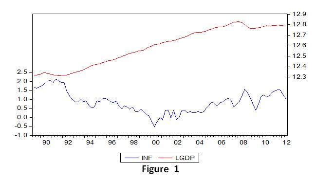
Figure 1 shows the trend of inflation and LGDP. In 1991:3 LGDP reaches its lowest point, probably because of the recession in the UK and the global recession, whereas inflation reaches its maximum. From then on, LGDP increased, making the UK’s economy one of the strongest in terms of inflation, which remained relatively low. In 2008, however, when another recession began, there was an enduring drop in LGDP, starting from 2008:1 until 2009:2, making this recession the longest so far, with inflation decreasing. Finally, the UK economy started improving in 2009:4. In general, it seems that although inflation is negatively related to LGDP, it has also a small effect on changes in LGDP. From these plots, a trend in LGDP is apparent, so we can assume that LGDP may be unit root with stationary drift or trend. On the other hand, there is no apparent trend in inflation and thus we might infer that inflation is either stationary around the mean or, at most, a drift-less unit root process. However, these will be checked later by doing the unit root test.
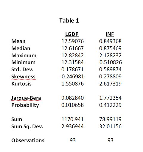
Table 1 below illustrates the descriptive statistics of these variables. We see that inflation is more spread out than LGDP, because its standard deviation is higher (0.589>0.178), implying that inflation is more volatile than LGDP. Moreover, LGDP has a left-skewed distribution (-0.246981<0), whereas inflation has a right-skewed distribution (0.278809>0). Both variables have a platykyrtic distribution, flatter than a normal with a wider peak (LGDP: 1.550876<3, INF: 2.617319<3).
4) Methodology
Most of the theories imply that there is a negative relationship between inflation and GDP. In this section we will estimate empirically the impact of inflation on GDP using the following ad-hoc relationship:
LGDP = β0 + β1 INF + et (1)
where β1 represents the long run elasticity with respect to inflation.
4.1) Unit root test:
First, we have to check the order of integration of our variables. We want them to be stationary, because non-stationarity leads to spurious results, since test statistics (t and F) are not following their usual distributions and thus standard critical values are almost always incorrect. Using the augmented Dickey-Fuller (ADF) test, we can distinguish between non-stationary processes and stationary processes with the null hypothesis as there is a unit root (H0: c3=0). From the Figure 1 above we see that inflation doesn’t have trend, and therefore we are doing the test using only intercept, whereas for LGDP we do the test using both trend and intercept. The test shows that both variables are non-stationary and integrated of order 1 (I(1))[2].
In order to make our variables stationary we have to de-trend the variables. In order for our variables to be de-trended, we generate their first differences. Therefore, when we do the test for the de-trended variables we use only the intercept choice. Now the variables are stationary and integrated of order 0 (I(0))[3]. The results are summarised in Table 2.
Table 2
Summary of ADF Test Results
| Series | Optimal Lag Length (SC) | ADF StatisticH0: c3=0 (unit root) | Inference |
| LGDP | 1 | -0.809312 | I(1) |
| ΔLGDP | 0 | -10.77312 | I(0) |
| INF | 0 | -1.977541 | I(1) |
| ΔINF | 4 | -9.535395 | I(0) |
The inference I(0) or I(1) is according to the 5% critical value.
Although we eliminated the trend by using the first differences, this will cause us to lose valuable and important information for the long run equilibrium. Therefore, Engle and Granger (1987) developed the co-integration analysis.
4.2) Long run analysis:
In this section we estimate our long-run model, showed in the equation (1) above, and then we test for co-integration in our variables by using the Engle-Granger approach. According to this approach, if the linear combination of non-stationary variables is itself stationary, then our series are co-integrated. We run the co-integration regression for (1), using both variables since they are non-stationary (I(1)) and then we test for the order of integration of the residuals.
The null hypothesis of this analysis is that our series are not co-integrated (H0: α1=0). We find that the t-statistic is -0.490 with MacKinnon p-value equal to 0.9636. Therefore, we accept the null hypothesis (H0) that our series are not co-integrated at the significance level of 5% (Table 3)[4]. Thus the residuals are non-stationary. Checking also for the residuals graph, they indeed appear to be non-stationary[5] and we cannot say anything about the long run relationship. However, we can say something about the short run. This is because, unlike the long run regression, the short run model contains I(0) variables, making the spurious problem much less likely.
Table 3
| Co-integration Test-Engel-Granger | Value | Probability* |
| Engel-Granger tau-statistic | -0.490242 | 0.9636 |
| Engel-Granger z-statistic | -0.635269 | 0.9767 |
* MacKinnon (1996) p-values
4.3) Short Run Analysis:
The model that we will use to estimate the short run relationship will be a dynamic ADL(5) model with the following form:
ΔLGDPt = φ + β0ΔINFt + β1ΔLGDPt-1 + β2ΔINFt-1 +β3ΔLGDPt-2 + β4ΔINFt-2 + β5ΔLGDPt-3 +
β6ΔINFt-3 + β7ΔLGDPt-4 + β7ΔINFt-4 + et (2)
In order to determine the number of lags in the model, we used the f +1 rule, where f is the frequency of the data. Since we have quarterly data, we start with an ADL(5) model. After estimating the short-run regression, we find that the only significant variables are ΔINF and ΔLGDPt-1 at the significance level of 5% [6]. So, we end up with the following parsimonious model:
ΔLGDPt = φ + β0ΔINFt + β1ΔLGDPt-1 + et (4)
The output of the regression shows that the coefficients of the ΔINFt and ΔLGDPt-1 have a negative (-0.005558) and positive (0.731485) impact on ΔLGDPt and they are both statistically significant at the significance level of 5% (Table 4). An increase in ΔLGDPt-1 of 1%, increases ΔLGDPt by 7.4%. However, an increase in ΔINFt of 1 %, decreases ΔLGDPt by 0.5 %. Thus, there is a negative relationship between inflation and GDP, as is expected to be found from the theory. Moreover, R2 shows that the model explains 52% of the variation of the data[7].
Table 4
Dependent variable: ΔLGDP
| Regressors | Coefficients | Standard error | t-statistic | p-value |
| Constant | 0.001282 | 0.000640 | 2.003360 | 0.0482 |
| ΔINF | -0.005558 | 0.002460 | -2.259701 | 0.0263 |
| ΔLGDP(-1) | 0.731485 | 0.074516 | 9.816434 | 0.0000 |
R2=0.52
When we do the diagnostic tests for the residuals, we see that they are ‘white noise’ at the significance level of 5%. More specifically, doing the LM test for serial correlation we see that the p-value is greater than 5%, so we cannot reject the null hypothesis of no serial correlation. In addition, the heteroskedasticity test shows that the p-value is again larger than 5% and thus the null hypothesis of homoskedasticity cannot be rejected. Finally, in the normality test, the p-value is smaller than 5%, so we can reject the null hypothesis for normality.
So, we see that our residuals are well-behaved, since they are consistent with no serial correlation and homoskedasticity, but they do not follow the normal distribution.[8] The results of these tests are summarized in the following table:
Table 5
Diagnostic Checking of the ADL(5) model
| H0: Residuals are . . . | Test | Test Statistic | p-value |
| Normally distributed | Bera-Jarque | 7.850061 | 0.0197 |
| Serially uncorrelated | Breusch-Godfrey | 0.209931 | 0.6468 |
| Homoskedastic | Breusch-Pagan-Godfrey | 4.786648 | 0.0913 |
5) Conclusion
The aim of this study was to test the relationship between inflation and GDP in the United Kingdom. Before we estimate this relationship we checked the order of integration of the variables. Both variables were non-stationary and integrated of order 1 (I(1)). The Engle-Granger test shows that they are also not co-integrated. Therefore, we cannot say anything about the long run equilibrium. Thus, we used a dynamic short-run model, which consists only of stationary variables and hence there are not any spurious problems. The residuals of this model are well-behaved and their properties are consistent with the assumptions of Gauss Markov.
Finally, we can see that there is a negative relationship between inflation and GDP in the United Kingdom, at least in the short run, which is consistent with most of the theories that have been developed throughout the years.
6) References:
- Fischer S. (1993) “The Role of Macroeconomic Factors in Growth”, Journal of Monetary Economics, Vol. 32, pp. 45-66.
- Barro R. (1995) “Inflation and Economic Growth”, Federal Reserve Bank of St. Louis Review, Vol. 78, pp. 153-169.
- Bruno, M. and Easterly, W. (1996) “Inflation Crises and Long-Run Growth”, Review of Federal Reserve Bank of St. Louis, Vol. 78, no. 3, pp. 139-46.
- Ghosh A. and Phillips S. (1998) “Warning: Inflation May be Harmful to Your Growth”, IMF Staff Papers, Vol. 45, pp. 672-710.
- Engle RF, Granger CWJ (1987) “Co-integration and error correction: representation, estimation and testing”, Econometrica, Vol. 55, pp. 251-276.