Computational Fluid Dynamics
Nomenclature
Re = Reynolds Number
ρ = Air Density
v = Velocity
V = Aircraft Velocity
M = Mach Number
a = Speed of Sound
α = Angle of Attack
L = Characteristic Length
c= Chord Length
µ = Kinematic Viscosity
Objectives
- To critique CFD results achieved in assignment one. The focus of the critique will be on mesh quality and results accuracy.
- To use the critique to demonstrate areas of improvement showing the improvements where applicable.
- To evaluate the group performance and recommend improvements where possible.
Introduction
This report will be split into the three objectives explained above. Each objective will be discussed in separate section headings. Concise observations from the first objective will be made and utilised as a means of improving the quality of the CFD aerofoil model. These will form the areas of improvement that will satisfy the second objective.
The second objective will be the main bulk of the report as the weaknesses exposed for analysis of assignment one will be improved upon. The improvements will be shown by means of screen shots to be explained and analysed in relation to the CFD model.
The final section of the report will focus on the third objective and will be a brief critical analysis of the group dynamics and what may have been done differently if the assignment was attempted again.
1.0 Critique of Assignment One
Section one will critically analyse the methods used in assignment one to find areas of improvement. The meshing method will be assessed first.
1.1 GAMBIT
GAMBIT software was used for meshing the NACA 4412 aerofoil in assignment one. The mesh is illustrated in figure 1.
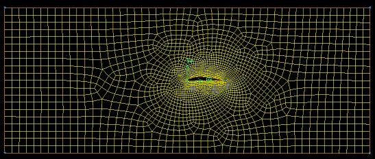
Figure 1 – Assignment one mesh of NACA 4412 aerofoil
Figure 1 shows the mesh of the aerofoil. Further research into aerofoil meshing techniques and lectures given has shown that the mesh does not provide the required accuracy to explain the airflow behaviour around the aerofoil and in particular drag (Lodgson, 2006).
The magnitude of pressure drag increases with the angle of attack due to a larger surface area for the airflow to act against which causes flow separation (see figure 2). At higher angles of attack the aerofoil changes from a streamlined body to a blunt body in aerodynamic terms. Therefore, a finer mesh is required around the areas where the flow is in-viscid to provide a more accurate analysis of the drag effects.
This concept is illustrated in figure 2. As can be seen, the pressure drag increases as the angle of attack does.
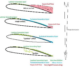
Figure 2 – An illustration of the increase in pressure drag
At low angles of attack the drag is caused by frictional drag by the contact on the boundary layer and the aerofoil skin.
1.2 Analysis of Fluent Results
Research into aerofoil CFD modelling has shown that the correct methods were not followed in setting up the boundary conditions and the lift and drag forces acting on the aerofoil. This gave the assignment one results a higher margin for error as the drag effects were not adjusted for an altering angle of attack. This meant that as α changed, the drag was still set as if α was 0°. Lift acts perpendicular to the aerofoil chord line and this was not adjusted at all in assignment one. The methods for including the lift and drag components will be included in section two (Bhaskaran, 2009).
Upon reflection of the screenshot explanation, the physical characteristics effecting lift and drag were poorly explained. This will be rectified in section two by explaining how the airflow behaviour affects both phenomena.
The results gained from assignment one were found to be inaccurate due to the above parameters. In order to ensure that the results retain accuracy, existing aerofoil data from wind tunnel testing will be analysed. This will give an excellent comparison opportunity and show how accurate the CFD modelling was.
2.0 Areas of Improvement
The areas taken from section one for re-modelling will form section headings and was:
- Mesh Size and Quality
- Accuracy of Results in Fluent
- Result Comparison.
2.1 Mesh Size and Quality
The mesh was re-started to ensure that a more accurate area of analysis was based around the aerofoil section.
The stages are described below:
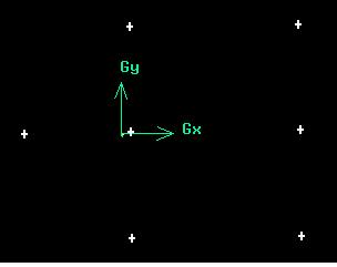
Figure 3 – Vertices plotted on GAMBIT
- The co-ordinates in table 1 (see appendix 1) were used to plot the vertices for the aerofoil shown in figure 3.
- The vertices were joined up to form the edges of the mesh.
As can be seen from figure 4, the edges make up three shapes allowing a finer mesh to be established around the aerofoil.
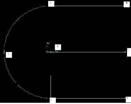

Figure 4 – The faces for meshing - Faces were created from the edges to enable the mesh to be completed. This enabled different meshes to be created in each face. The mesh around the aerofoil was created by splitting the edges at 0.3c. This gave a finer mesh around the leading edge and the area above and below the wing where the dynamic pressure can be monitored for drag effects. (See appendix 2 and 3 for the mesh parameters.)
- The final mesh is shown below.
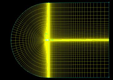
Figure 5 – The final mesh
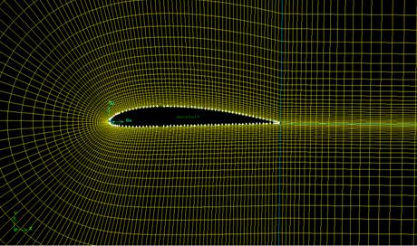
Figure 6 – Zoomed in view of the mesh
As can be seen from figures 5 and 6 the mesh is finer around the aerofoil and the mesh takes into account the pressure distribution above and beneath the wing.
As can be seen from figure 6, the mesh is uniformly spread around the aerofoil with an adequate growth rate that provides a higher degree of accuracy than the mesh used in assignment one shown in figure 1.
This was achieved by splitting the top edge of the aerofoil shown in figure 6.
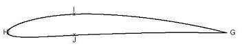
Figure 7 – An aerofoil image showing how the edges were split (Bhaskaran, 2009). See appendix 3 for the mesh parameters.
2.1.1 Learning Outcomes:
- To use co-ordinates as vertices for the mesh outline
- To create edges from vertices and edges to faces
- To mesh individual faces with different mesh parameters along edges
- To split edges to create a finer mesh. 0.3c was used to split the edges
- To mesh an aerofoil with the required fineness in the area where the airflow is most disturbed.
2.2 Fluent Results
The same mesh was used for each set of results. The boundary conditions were standard seal level conditions shown below.
Standard Sea Level Conditions were assumed
Density = 1.225 kg/m3
Pressure = 101, 325 Pa
Temperature = 288.15 K
Re = ρ V L / µ
= 1.225 * 78 * 1 / 13.3 * 10-6 = 7.2 * 105.
The lift and drag force parameters were changed to compensate for the changing angle of attack. This was achieved for α = 4 by the x velocity = 77.8m/s and the y velocity = 5.4 m/s. The lift force in the x direction was -0.698 and the y direction 0.998. The drag component was 0.998 in the x direction and 0.0697 in the y direction. This procedure was followed as α changed to 16°.
The results are recorded below.
| Angle of Attack ˚ | CL | CD |
| 0 | 0.24 | 0.01 |
| 4 | 0.51 | 0.028 |
| 8 | 0.835 | 0.14 |
| 12 | 1.15 | 0.16 |
| 16 | 1.28 | 0.21 |
| Angle of Attack ˚ | CL | CD |
| 0 | 0.36 | 0.01 |
| 4 | 0.61 | 0.04 |
| 8 | 0.85 | 0.07 |
| 12 | 1.05 | 0.12 |
| 16 | 1.18 | 0.16 |
| Angle of Attack ˚ | CL | CD |
0 | 0.3 | 0.014 |
4 | 0.68 | 0.016 |
8 | 0.95 | 0.027 |
12 | 1.15 | 0.092 |
16 | 1.2 | 0.15 |
The accuracy of the imported mesh was refined by lowering the y-plus values to enable a more accurate set of results to be gained. The mesh was refined as the process of the first order results were carried out. The parameters for the drag, the lift and x and y velocity components were changed in fluent as shown above.
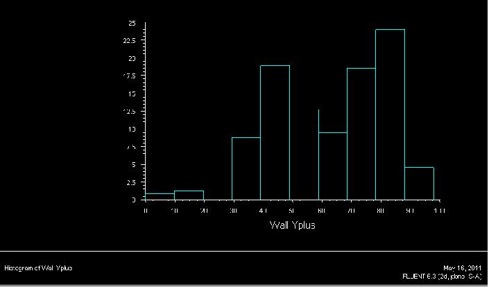
Figure 8 – The histogram of y-plus values
Graph 1 shows the lift coefficients of the results in tables 5, 6 and 7. As can be seen, there was an improvement in accuracy when the solver ran from the first order to the second order. Up to α = 8, the second order show a similarity to the existing NACA 4412 data. However, the aerofoil did not stall on the CFD results as it is shown in the existing data.
The first order results show a level of inconsistency as it interests the existing data line when α = 13. The first order results interest the second order results line when α = 9. This has shown the importance of running through the results on the first and second order to improve the accuracy of the lift coefficient.
Although the lift coefficient does not level off when α = 12 as the existing results do, the line shows that the lift coefficient is reducing which may result in the stall of the aerofoil if further angles of attack were tested. The maximum difference between the two coefficients was 0.1 and the minimum difference was 0.02. The average difference was 0.07 between the existing results and the second order ones. The difference shows there are errors. This could be due to the outer area of the mesh not being fine enough to account for all the lift forces. However, the mesh was a distinct improvement from assignment one. Sources of error are expected from CFD software when compared to that of existing data.
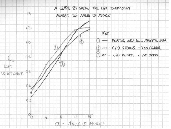
Graph 1 – The lift coefficient and α
Graph 2 shows the drag coefficients of the tables 5, 6 and 7. As can be seen the first order, results were inaccurate. The final drag co-efficient was not plotted as it was 0.21 which would have meant applying a smaller scale to the graph. They show reasonable accuracy when α = 0 and 4. However, the drag coefficient gets further away from the existing data as α is increased.
The second order results show a similar shape in terms of the line to the existing results and the accuracy of the drag improves as α increases. The average difference between the second order and existing results is 0.015. The mesh was within the required y + values but CFD software has difficulties with creating the turbulent flow that causes drag. This could be a reason for the source of error. From the first order to the second order the results became more accurate. With a higher knowledge of Fluent the results for both the lift and drag may have been improved even more.
The results are satisfactory as they show similar characteristics in terms of accuracy. It has been shown how it is significant that the results are run through on the second order as there is a big difference on graphs 1 and 2 in accuracy.
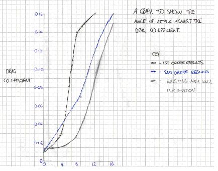
Graph 2 – Drag coefficient against α
2. 3 Drag and Lift
Lift is generated by the pressure distribution over the top of the aerofoil.
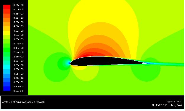
Figure 9 – Pressure distribution when α = 0
Figure 9 shows the pressure distribution over the wing. The difference between the upper and lower aerofoil create the lift. The drag at low angles of attack is due to the skin friction created by the airflow passing over the aerofoil. This is called the boundary layer.
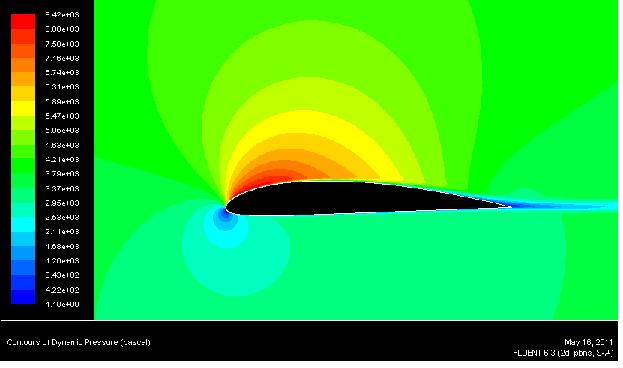
Figure 10 – Pressure distribution when α = 8.
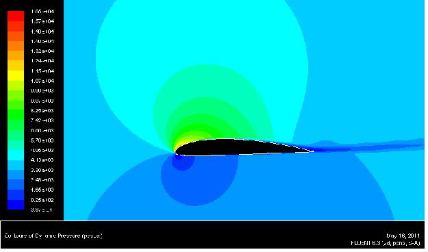
Figure 11- Pressure distribution when α = 16
At low angles of attack, the drag acting on the aerofoil is caused by skin friction between the air and the upper aerofoil surface. The layers of air at the surface stop moving and the layers or air increase in velocity the further away from the surface they are. The drag results from shear stresses acting between the boundary layer and the upper aerofoil surface (Kermode, 2006).
At higher angles of attack, the airflow acting over the aerofoil begins to separate. This is called the transition point. An analysis of figures 9, 10 and 11 shows the transition point moving forward as the boundary later separates. The shear stress acting on the boundary layer creates less drag and the dominant drag force is the pressure drag. Pressure drag is caused by the pressure difference between the front and rear of the aerofoil. As the aerofoil creates more lift there is a higher pressure distribution above the wing which is shown in figure 10. This increases the pressure drag which is illustrated in graph 2 by the resultant increase in the drag coefficient (Young et al., 2011).
This section will reflect on the individual and group work completed in semesters one and two.
3.0 Group Work
The group gained three different sets of results based around the analysis of an aerofoil. In that respect the objectives were achieved. Having had no experience on CFD software, it was a learning process from day one of the first semester. The first idea was to use a plane modelled by the group for analysis. However, the geometry was too complex to be able to mesh and GAMBIT crashed when the mesh was applied. This early experience served the group well as it showed the limitations and from that we decided to keep the modelling simple and in two dimensions.
Each member chose different methods of analysis of an aerofoil which gave the group more information and experience to learn from as ideas were exchanged on different ways of meshing and using Fluent. The group worked well together and the dynamics were excellent as no member was left out of any decision or process. The experience of working in a group on other modules helped as each member trusted the other two to keep up with the required work.
3.1 Individual Work
The opportunity to re-correct work from assignment one proved to be invaluable and taught how to use GAMBIT and Fluent features in a higher depth. The process of re-reading assignment one and comparing the existing techniques used for aerofoil analysis was useful as it presented various errors. The process of re-meshing the aerofoil and adding the missing drag and lift parameters has shown various functions of GAMBIT and Fluent that can only be learnt from performing the mesh. The knowledge acquired was slow at the beginning of the year due to the software being new. However, after semester one was completed, the knowledge base on the subject grew. This is shown by the mesh used for the aerofoil in assignment two. The lift and drag parameters were set up correctly, which produced a good model for analysis.
The method of extracting the correct data from Fluent was improved from assignment one to assignment two. In assignment one, the screenshots were shown and described. However, assignment two improved upon this by plotting the lift and drag coefficients and comparing against existing data. The physical characteristics of drag generation were explained to show a wider knowledge of how the airflow reacts against the aerofoil surface.
Overall the refined method used for assignment two was more time consuming; however, more knowledge was gained from this process.
References
Bhaskaran, (2009), Flow over an Aerofoil, Cornell University, [online] Available from
https://confluence.cornell.edu/display/SIMULATION/FLUENT+-+Flow+over+an+Airfoil-+Problem+Specification, Accessed on 10/05/2011
Bhaskaran, (2009), Flow over an Aerofoil, Cornell University, [online] Available from
https://confluence.cornell.edu/display/SIMULATION/FLUENT+-+Flow+over+an+Airfoil-+Step+2, Accessed on 10/05/2011
Kermode, A, (2006), Mechanics of Flight, 11th Edition, Pearson Education Limited.
Logsdon, N, (2006), A Procedure for Numerically Analysing Aerofoils and Wing Sections, University of Missouri, [online] Available from http://web.missouri.edu/~solbrekkeng/TherMMEC/pubs/thesis_logsdon.pdf, Accessed on 11/05/2011
Xin et al., (2010), Numerical Simulation and Aerodynamic Performance Comparison between Seagull Aerofoil and NACA 4412 Aerofoil under Low Reynolds, Advances in Natural Science, Vol 3 No 2, pp 244 – 250 [online] Available from http://www.cscanada.net/index.php/ans/article/viewFile/1422/1596, Accessed on 15/05/2011
Young et al., (2011), A brief Introduction to Fluid Mechanics, Fifth Edition, Wiley Publications.
Bibliography
Princeton University, nd, Drag of Blunt and Streamlined Bodies, [online] Available from
http://www.princeton.edu/~asmits/Bicycle_web/blunt.html, Accessed on 12/05/2011
Potter, M, (2009), Fluid Mechanics – De-Mystified, McGraw Hill,
Rotary Forum, (2011), The Decrease in Pressure Drag, [online] Available from
http://www.rotaryforum.com/forum/showthread.php?t=28842, Accessed on 12/05/2011
Appendices
Appendix 1
Label | X | Y | z |
A | c | 12.5c | 0 |
B | 21c | 12.5c | 0 |
C | 21c | 0 | 0 |
D | 21c | -12.5c | 0 |
E | C | -12.5c | 0 |
F | -11.5c | 0 | 0 |
G | C | 0 | 0 |
In reference to table 1, c = chord length = 1m. Therefore 12.5c = 21 * 1 = 12.5m
Appendix 2
Edges | Successive Ratio | First Length | Interval Count |
GA, BC, EG, CD | 1.15 | X | 45 |
AB, CG, DE | X | 0.02c | 60 |
Appendix 3
Edges | Last Length | Successive Ratio | Interval Size | Interval Count |
HI, HJ | 0.02c | x | x | 40 |
IG, JG | x | 1 | 0.02c | x |
Edges | First Length | Interval Count |
AF, EF | 0.02c | 75 |