The operation and the applications of genetic algorithms.
Abstract
This report describes the use of the operation and the applications of genetic algorithms. It describes the development and the application phases of the desired algorithms. The advantages of using the genetic algorithm as the solution finding methods are also shown. The formation of the fitness function and the other genetic operators is also discussed in this report. This report is concluded by the discussion on how successfully the genetic algorithms are being used in the different applications and the significance they make in the performance of modern advance equipment.
1 Introduction
What are genetic algorithms?
Genetic algorithms are actually the generalized form of Darwin’s theory of evolution.
These algorithms are numerical optimization algorithms inspired by both natural selection and natural genetics. This is a general method which can be applied to a number of problems. The theory of these algorithms is easy to understand and to put into coding for the solution of a variety of problems.
Why use genetic algorithms?
The genetic algorithms are a robust technique to perform the complex calculations and to estimate a series of unknown parameters within a physical system.
What are genetic operators?
These are the operations performed on a randomly generated population of strings. These strings are also called ‘chromosomes’, because the genetic operators applied on them are similar to those applied on biological chromosomes. These genetic operators are used to maintain the genetic diversity.
2. Genetic algorithms
In this chapter, genetic algorithms are introduced, what they are, from where they evolved and how they are compared to and differ from other search procedures.
2.1 Introduction to genetic algorithms
Genetic algorithms are search algorithms based on mechanics of natural selection and natural genetics. These algorithms are the method used to find out approximate solutions to complex problems through the application of principles of evolutionary biology to computer science. These algorithms are a particular class of evolutionary algorithms. Genetic algorithms are typically implemented as a computer simulation in which a population of abstract representations (called chromosomes) of candidate solutions (called individuals) to an optimization problem evolves toward better solutions. Normally, solutions are represented in binary as strings of 0s and 1s, but different encodings are also possible. The evolution starts from a population of completely random individuals and happens in generations. In each generation, the fitness of the whole population is evaluated, multiple individuals are stochastically selected from the current population based on their fitness and are modified (mutated or recombined) to form a new population, which becomes current in the next iteration of the algorithm.
In every new generation, a new set of chromosomes (strings) is created using the fittest parts of the old; an occasional new part is tried for good measure.
2.2 Operation of genetic algorithms
It is very important to understand the workings of the genetic algorithms in order to use them efficiently. Since the problems are handled as a computer program and the problem in defined in the form of a computer code , the problem to be solved is represented by a list of parameters which can be used to drive an evaluation procedure, called chromosomes or genomes. Chromosomes are typically represented as simple strings of data and instructions.
Initially, several such parameter lists or chromosomes are generated. This may be totally random, or the programmer may define a method to form the initial parameter chromosomes or strings. This is called the ‘first generation’.
During each successive generation, each individual string is evaluated, and a value of how good an individual is or the fitness value is returned by a ‘ fitness function’. The pool is sorted, with those having better fitness representing better solutions to the problem ranked at the top. It is not necessary that in a generation there must be a string that is ranked the best as a solution but for that generation only. It is likely that we get the results that are not good solutions as required.
The next step is to generate a second generation pool of organisms, which is done using any or all of the genetic operators: selection, crossover (or recombination) and mutation which will be discussed in detail in the coming sub-chapters. A pair of organisms is selected for breeding. Selection is biased towards elements of the initial generation which have better fitness, though it is usually not so biased that poorer elements have no chance to participate, in order to prevent the solution set from converging too early to a sub-optimal or local solution. There are several well-defined organism selection methods which will be explained later in this chapter.
Following selection, the crossover operation is performed upon the selected chromosomes. A random number between 0 and 1 is generated, and if it falls below the crossover threshold, the organisms are mated; otherwise, they are propagated into the next generation unchanged. Crossover results in two new child chromosomes, which are added to the second generation pool. The chromosomes of the parents are mixed in some way during crossover. This process is repeated with different parent organisms until there are an appropriate number of candidate solutions in the second generation pool.
The next step is to mutate the newly created offspring. Normally genetic algorithms have a fixed, very small probability of mutation. A random number between 0 and 1 is generated; if it falls within the Pm range, the new child organism’s chromosome is randomly mutated in some way, typically by simply randomly altering bits in the chromosome data structure. Usually the mutation is very unlikely to occur but it is a very important genetic operator used to maintain the genetic diversity from one population of chromosomes to the other.
These processes ultimately result in a second generation pool of chromosomes that is different from the initial generation. Generally the average degree of fitness will have increased by this procedure for the second generation pool, since only the best organisms from the first generation are selected for breeding. The entire process is repeated for this second generation: each organism in the second generation pool is then evaluated, the fitness value for each organism is obtained, pairs are selected for breeding, a third generation pool is generated, etc. The process is repeated until an organism is produced which gives an adequate solution.
A slight variant of this method of pool generation is to allow some of the better organisms from the first generation to carry over to the second, unaltered. This form of genetic algorithm is known as an ‘ elite selection strategy’.
2.3 Genetic operators
A genetic operator is a process used in genetic algorithms to maintain genetic diversity.
Genetic variation is a necessity for the process of evolution. Genetic operators used in genetic algorithms are analogous to those which occur in the natural world: survival of the fittest, or selection; asexual or sexual reproduction cross over or recombination; and mutation.
2.3.1 Selection
The basic principle of the selection is to give preference to better individuals, allowing them to pass on their genes to the next generation. The goodness of each individual depends on its fitness. Fitness may be determined by an objective function called a ‘ fitness function’.
As we already know, chromosome are selected from the population to be parents to perform crossover. The problem is how to select these chromosomes. According to Darwin’ s theory of evolution, only the best ones should survive and create new offspring. There are many methods used to select the best chromosomes; for example: roulette wheel selection; Boltzman selection; tournament selection; rank selection; and steady state selection.
2.3.1. a . Roulette wheel selection
In this type of selection the parent strings are selected according to their fitness. The better the strings are, the better the chance of their selection. Roulette wheel selection is done by choosing the strings statistically based on their relative fitness values or simply the percentage. This concept can be easily understood by considering a roulette wheel where all chromosomes of the population are placed. They are given the space on the wheel according to their fitness values. So if a dice is thrown on the roulette wheel, the probability of the fitter chromosome to occur is greater than the other population members.
| String number | String | Fitness | Percentage of total |
| 1 | 10110000 | 3 | 21.4 |
| 2 | 01101110 | 5 | 35.7 |
| 3 | 00100000 | 1 | 7.2 |
| 4 | 01101110 | 5 | 35.7 |
| Total | 14 | 100.0 |
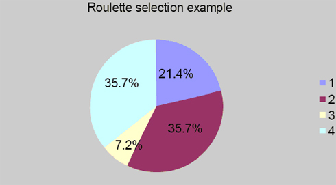
Figure 1: Representation of fitness according to table 2.1
2.3.1.b. Tournament selection
Using the tournament selection requires usually two individuals,which are picked up randomly from the population. From these two individuals,the fittest individual is selected by the probability given by:
Probability = (1+r)/2
where r is a random number between 0 and 1. The fitter of the individuals forms the parent string. Binary tournament selection can be regarded as performing ranking selection with a roulette wheel sampling, and it is one of the most commonly used techniques in genetic algorithm applications.
2.3.1. c. Rank selection
The previous selection will have problems if the fitness differs greatly. For example, if the best chromosome fitness is 90 percent of the entire roulette wheel then the other chromosomes will have very few chances to be selected. Rank selection first ranks the population and then every chromosome receives fitness from this ranking. The worst will have fitness 1, second worst will have 2 etc. and the best will have fitness N (where N is the number of chromosomes in the population). After this, the chromosome has the chance to be selected. But this method can lead to slower convergence, because the fittest chromosome does not differ much from the other chromosomes.
2.3.2 Fitness function
The fitness function is a particular type of function which quantifies the optimality of a solution, which is a chromosome in our case since we are using genetic algorithms, so that the particular chromosome may be ranked against all the other chromosomes. Optimal chromosomes, or at least chromosomes which are more optimal, are allowed to breed and mix their data sets by any of several techniques, producing a new generation that is expected to be even better.
An ideal fitness function correlates closely with the algorithm’s goal, and yet may be computed quickly. Speed of execution is very important, as a typical genetic algorithm must be iterated many, many times in order to produce a usable result for a complex problem.
2.3.3 Crossover
In genetic algorithms, crossover is a genetic operator used to vary the programming of a chromosome or chromosomes from one generation to the next. It is an analogy to reproduction and biological crossover, upon which genetic algorithms are based. Most genetic algorithms have a single adjustable probability of crossover, typically between 0.6 and 1.0, which encodes the probability that two selected organisms will actually breed. Many crossover techniques exist for organisms which use different data structures to store themselves.
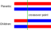
One-point crossover
A crossover point on the parent strings is selected. All data beyond that point in the parent strings is swapped. The resulting strings are the children. The following figure shows the single point crossover.
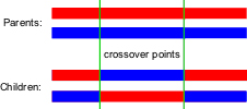
Two-point crossover
Two-point crossover calls for two points to be selected on the parent organism strings. Everything between the two points is swapped between the parent organisms, rendering two child organisms:
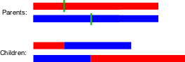
Cut and splice
Another crossover variant, the ‘cut and splice’ approach, results in a change in length of the children strings. The reason for this difference is that each parent string has a separate choice of crossover point.
Uniform crossover and half uniform crossover
In both these schemes, the two parents are combined to produce two new offspring.
In the uniform crossover scheme, individual bits in the string are compared between two parents. The bits are swapped with a fixed probability,typically 0.5.
In the half uniform crossover scheme, exactly half of the non-matching bits are swapped. Thus, first the Hamming distance (the number of differing bits) is calculated. This number is divided by two. The resulting number is how many of the bits that do not match between the two parents will be swapped.
2.3.4 Mutation
In genetic algorithms, mutation is a genetic operator used to maintain genetic diversity from one generation of a population of chromosomes to the next. It is analogous (similar) to biological mutation.
The classic example of a mutation operator involves a probability that an arbitrary bit in a genetic sequence will be changed from its original state. A common method of implementing the mutation operator involves generating a random variable for each bit in a sequence. This random variable tells us whether or not a particular bit will be modified.
The purpose of mutation in genetic algorithms is to allow the algorithm to avoid local minima by preventing the population of chromosomes from becoming too similar to each other, thus slowing or even stopping evolution. This reasoning also explains the fact that most genetic algorithm systems avoid only taking the fittest of the population in generating the next, but rather a random or semi-random selection with a weighting toward those that are fitter. Typical genetic algorithms have a fixed, very small probability of mutation of perhaps 0.01 or less.
2.3.5 Elitism
This is a very important function of genetic algorithms. When the genetic algorithms create a new population, there is a great chance that they might lose the best individuals. By the use of elitism, the best solutions are first copied into the new generation and then the rest of the process follows the normal procedure.
2.4 Why use genetic algorithms?
The methods described above are purely inspired by real genetics. Although genetic algorithms are very robust techniques for solving optimization problems (that is seeking improvement to approach an optimal point), there has not been much investigation by scientists into why it works and to what degree the crossover and mutation operators improve genetic algorithm performance over a large set of applications. Genetic algorithms are considered to be evolving computer programs. This is closely coupled with artificial intelligence used in many computer applications today, since it seems that genetic algorithms learn from them and find the optimum solution as the processing time passes. Genetic algorithms offer robustness and reliability to artificial systems, hence eliminating costly redesigns. Some advantages of using genetic algorithms for optimization problems is that they are resistant to becoming trapped in local optima and that they search globally for a solution using the fitness function values for optimization. The major disadvantage of genetic algorithms is that they have trouble finding the exact global optimum and that they require a large number of fitness function evaluations.
2.4.1 Comparison of genetic algorithms with the usual methods
The following list is a brief look at the essential differences between genetic algorithms and other forms of optimization.
- Genetic algorithms use a coded form of the function values (parameter set), rather than the actual values. They use the binary strings representing the variables. So the genetic algorithms do not search the problem space using the traditional values of the variables, instead they use the binary strings representing the variables.
- Genetic algorithms use a set of strings, or populations, of points to carry out a search towards the solution of certain problem space, not just a single point on that problem space.This is why the genetic algorithms are able to provide the optimum solution in complex and quite noisy spaces where there are a lot of local optimal points. Normally, the traditional methods rely on the single point value to search through the work space.Genetic algorithms use a set of values, so they have a better view of the problem space, and hence provide the optimal solution.
- In problem solving, the traditional methods need variety of information to work on the problem. Genetic algorithms use only the initial information before solving the problem . Once the genetic algorithm gets a measure of fitness about a point in the problem space,it guides itself towards the optimized solution.
- Unlike other optimization methods, genetic algorithms are probabilistic in nature. They are not deterministic like other traditional methods.
- Genetic algorithms have a natural parallel execution of strings or we can say that they are inherently parallel.They deal with a large number of strings at the same time. It is estimated that genetic algorithms process N numbers of strings at one time, but in actual practice genetic algorithms are processing 3N useful sub- strings.
2.5 Limitations of genetic algorithms
The genetic algorithms as described above are very flexible yet they have some limitations. These limitations are discussed as follows:
- The number of chromosomes in a population can neither be too large nor too small. When we initialize the population and the population size is too small, the algorithm is left with very small search space or simply with fewer options for the solution. If the population size is too large, this results in a much increased number of generations, hence increased processing in each generation. This greatly increases the processing time for each generation. So the generation size of 50 –100 is recommended.
- The probabilities for the crossover and the mutation functions are defined as constants. These probabilities play an important role in maintaininggenetic diversity. So bearing a change in these probabilities is not desired as they can induce instability in the developed system. This, however, does not mean that they are the best values for the system but it is better not to change the preset values for the developed system. The recommended crossover probability is from 0.8 to 0.95 and the recommended values for the mutation probability are from 0.005 to 0.01. The values between the ranges defined above do not affect the performance of the system much and therefore are acceptable.
- Another major limitation of genetic algorithms is that they have trouble finding the exact global optimum and that they require a large number of fitness function evaluations.
3 Applications
Genetic algorithms have evolved as a very effective method in artificial intelligence design and automated design. The applications of these algorithms are listed below.
- Artificial creativity.
- Automated design, including research on composite material design and multi-objective design of automotive components for crashworthiness, weight savings, and other characteristics.
- Automated design of mechatronic systems using bond graphs and genetic programming (NSF).
- Automated design of industrial equipment using catalogues of exemplar lever patterns.
- Calculation of bound states and local-density approximations.
- Chemical kinetics (gas and solid phases).
- Configuration applications, particularly physics applications of optimal molecule configurations for particular systems like C60 (buckyballs).
- Container- loading optimization.
- Code-breaking, using the genetic algorithmsto search large solution spaces of ciphers for the one correct decryption.
- Design of water distribution systems.
- Distributed computer network topologies.
- Electronic circuit design, known as ‘evolvable hardware’.
- File allocation for a distributed system.
- JGAP: Java Genetic Algorithms Package, also includes support for Genetic Programming.
- Parallelization of genetic algorithms /geneticprogrammesincluding use of hierarchical decomposition of problem domains and design spaces, nesting of irregular shapes using feature matching and genetic algorithms .
- Game Theory Equilibrium Resolution.
- Learning robot behaviour using genetic algorithms.
- Learning fuzzy rule base using genetic algorithms.
- Linguistic analysis, including Grammar Induction and other aspects of Natural Language Processing (NLP), such as word sense disambiguation.
- Mobile communications infrastructure optimization.
- Molecular Structure Optimization (Chemistry).
- Multiple population topologies and interchange methodologies.
- Optimization of data compression systems, for example using wavelets.
- Protein folding and protein- ligand docking.
- Plant floor layout.
- Representing rational agents in economic models such as the cobweb model.
- Scheduling applications, including job-shop scheduling. The objective being to schedule jobs in a sequence dependent or non-sequence- dependent setup environment in order to maximize the volume of production while minimizing penalties such as tardiness.
- Selection of optimal mathematical model to describe biological systems.
- Software engineering.
- Solving the machine-component grouping problem required for cellular manufacturing systems.
- Tactical asset allocation and international equity strategies.
- Timetabling problems, such as designing a non-conflicting class timetable for a large university.
- Training artificial neural networks when pre-classified training examples are not readily obtainable (neuroevolution).
- Travelling Salesman Problem.
- MMIC impedance matching systems.
- Input impedance antennaautomatic matching system.
- Automatic impedance matching of an Active Helical Antenna Near a Human Operator.
- An automatic impedance matching system for a multi-point power delivery continuous industrial microwave oven.
4 References and Bibliography
Horrocks, D. H. and Spittle, M. C., Genetic Algorithms, IEE Colloquium on Circuit Theory and DSP, Feb 1992 (London), pp 1–4
Goldberg, D. E., Genetic Algorithms in Search, Optimization and Machine
Learning, Addison-Wesley 1989, pp 1–25, 61–88, 217–265
Mitchell, M., An Introduction to Genetic Algorithms, MIT Press 1999 pp 171
David and Lawrence, Handbook of Genetic Algorithms, Van Nostrumd 1991
Sun Y. and Fidler, J. K., Design Method for Impedance Matching Networks, IEE Proc. Circuits Devices Systems, August 1996,Vol.143, pp 186–194
Sun Y., Lau, W. K., Antenna Impedance Matching using Genetic Algorithms, IEE National Conference on Antenna and Propagation, 1999, pp 31–37
Pitt, C.W, Sputtered Glass Optical Waveguides, Electronic Letters, 1973, 9 pp 401–403
Siau, J, et. al, Biometrics, Some Journal, 2005, pp 101–104
Websites
http://en.wikipedia.org/wiki/Genetic_algorithms
http://www.answers.com
http://www.uni-koblenz.de/~gb/projects/ale/studienarbeit_html/node19.html
http://www.rennard.org/alife/english/gavintrgb.html
Project reports
Al-Amoudi, Wideband Antenna Tuning and Impedance Matching using Genetic Algorithms, August 2002. University of Hertfordshire.
Broadband antenna tuning using Gas, 2003. University of Hertfordshire.
Yufei Ren, Broadband antenna tuning using genetic algorithms, April 2004 University of Hertfordshire.
Cheong kel Jun, Wideband tuning and impedance matching using genetic algorithms, April 2002. University of Hertfordshire.
Efthymios Sakelliou, Automatic Wideband Tuning of Impedance matching networks using genetic algorithms, August 2001. University of Hertfordshire.