Options Pricing Using Alpha Stable Volatility
Number of words: 5533
Data Collection and Study
The process of data collection is an involving process that involves a lot of precaution and assumptions. It involves understanding a summary of the roadmap to ensure the right data is collected. Throughout the process a lot of care and exemplary precision is put to ensure all data even though from different sources and time frames remains unison with the goal at hand. The data collected is critically visualized and using different modules is compared to each other ro ensure sanity and precision.
The first piece of data collected is that of the options to be sampled. Since the data is of the period of 2020, a good company to pick would be one heavily involved with the pandemic. 2020 was the year of reckoning for big Pharma and among these was Pfizer. Throughout the year Pfizer was at a constant spotlight from the Trump Government and the entire world as persons were waiting for the COVID-19 vaccine. The company did emerge as the first to make a production of the same but it faced challenges all together. Some of its competitors in the same field and market index include Johnson & Johnson, Merck & Co and Proctor & Gamble.
Having these facts as background information of the company was enough to settle for it as a choice in the analysis. The next factor that affected the dataset to be collected was the Time to Expiration of the option to be predicted. A common misconception among many analysts is that increasing the timeframe of the historical data of the stock price to be collected will improve the accuracy of the model. However, this is not always true. Data to far back can have little to no significant effect on the most recent data and thus the time frame should be well chosen. On the other hand, choosing a dataset with a smaller time frame will also mean constraining the predictability of the model, as such a way out needed to be found.
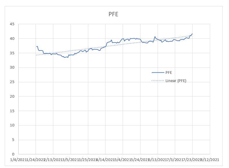
After sampling a great deal of literature addressing the same topic, a compromise of using the same time frame of historical stock prices as that of the time of expiration of the option to be predicted. Thus, having these two stock prices of Pfizer of a 180-day span from July 23rd were imported. The dated values started from January 25th 2021 to July 23rd 2021. The reason for this is because at the time of analysis the latest option announced by Pfizer was on July 23rd as can be seen from the screenshot below.
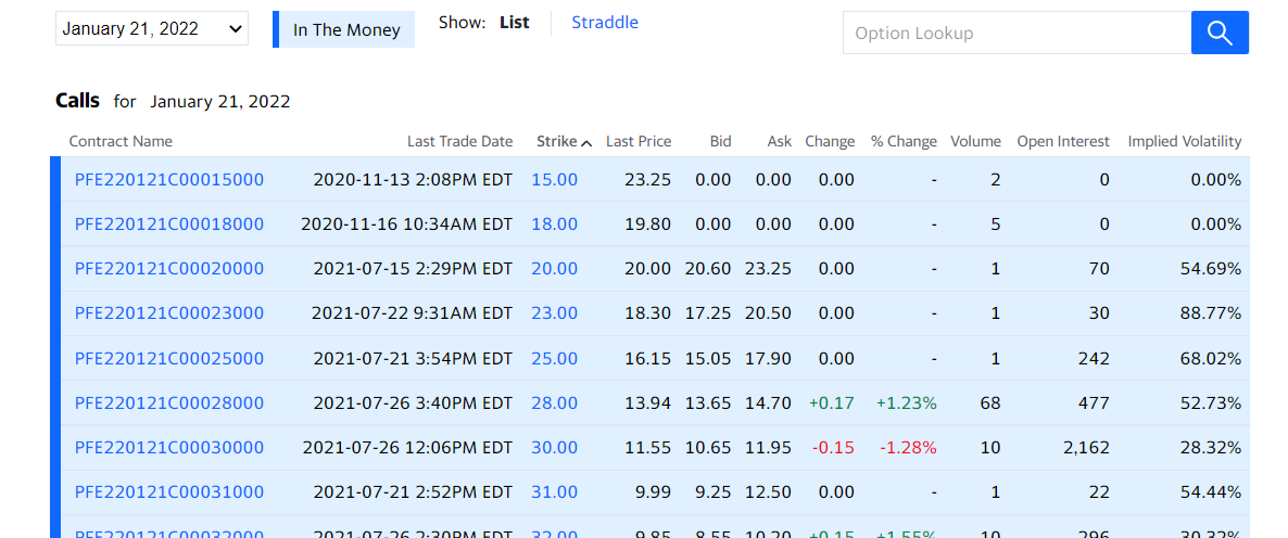
The 180-day chosen period will act as a precursor to the prediction of volatility of the stock. The next piece of data to be collected is that of the index associated to the Pfizer stocks. The index to be collected is the Dow Jones Industry Average, which consists of the top 30 blue chip corporations on Wall Street. The same timeframe is applied to the Dow Jones historical data portal and the dataset is downloaded. The resulting close prices are imported to the Pfizer historical prices data frame and stored beside. The next dataset to be collected is that that will provide a risk free rate. Now it is not true to affirm that government bonds and treasury bills are risky free assets, however their volatility is so minimal, they can be considered as risk-free assets. They lack the factors that surround a market or organization and thus can be considered a safe bet by most investors. The data is collected from the US Treasury website, the most effective coupons to use are the 26-week bills as they correspond to the sample period under analysis across the paper.
The required column is then copied and added to the main data frame having the closing prices of Pfizer and Dow Jones Index. The dates of the treasury bills are also ensured to be the same and the Independence Day of 4th July is also removed to ensure uniformity with stock dates. An if function is used to ensure that the dates of both the stocks and the T-bills are similar and the test turns out positive. The column names are then changed to ones that will be easier to use. The Pfizer and Dow closing prices are renamed as their company initials that is “PFE” and “DJIA” while the T-Bills are renamed to “rF”.
Having these three columns as the new dataset, makes it near complete. However, after a wide search for past prices of options, it is clear that very few to none of the financial web services, store historical prices of options. These include Washington post, Bloomberg, Google finance, Yahoo Finance, Investing.com and Weibull. This forces the model to be a prediction model instead of a causal one. However, this is not challenging as these companies provide estimations of the options prices calculated by other models such as Binomial, Trinomial and even the Black Scholes. Though not specified it is in line with this aspect and thus the model to be built using the new approach will try aiming for this goal and possibly predicting better that the ones available. The next phase involves data preprocessing which are the set of processes that make data ready for analysis and fitting into the model.
Data Preparation and Preprocessing
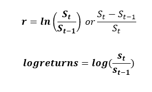
Data preprocessing as highlighted earlier is the gateway to building models and fitting data to models. It is a set of procedures that create, modify, delete, mutate and even change existing datapoints to create the necessary variables. The first thing to understand regarding historical data is that it is time-series. Thus, governed by a series of dates. Now according to the proposal, the first data to acquire from the dataset is the log returns of both the index and the underlying security. This is calculated by finding the natural logarithm of the division of previous closing stock price and the new closing stock price. Another methodology of finding the discrete returns is through dividing the change of new and old stock price in proportion to the old. The formulas of both methods are highlighted below. The r implementation is also shown beside it as it is quite similar:
The next procedure in the preprocessing stage is smoothing out the time frames. After calculation of the returns, it is clear that the latest date will not have its return as it is determined by the current’s stock price and the next stock price. This is an inconsistency that needs fixing. It will mean having a dataset that is not upright abd while we have 127 trading days, there is only 126 rerurns. The dataset should also be arranged in a manner that allows the oldest days to come first and the new ones next. Conversion of the log returns data frames to time series for exponential forecasting and fitting an Arima model is also done but this is just for finding support parameters which are not entirely important in the model to be built. The R implementation of this set of procedures is done using the dplyr package with functions such as mutate creating the new variables of PFEReturns and DJIAReturns, while the arrange function sorts the dataset following the dates column in an ascending manner, the na.omit() function removes any row that has missing data and thus the last row is removed from the dataset to achieve a dataset that is uniform and ready for processing. In a final spree, this will have us remaining with 5 columns and 126 days as rows.
On a regular basis, the preprocessing stage is the longest in the entire lifecycle of modeling, but since we are working with stock prices, the companies providing this data have done a lot into preprocessing to allow smooth plugging in of the data. There are even R packages such as Quandl which load the data straight into the R notebook with just a single request. This makes preprocessing easy and fast. He values to be calculated are also just simple binary functions such as addition, subtraction and division and thus even easier. Thus, in a summary, preprocessing such data is simple and does not require any complicated algorithms or methods. The next phase is the first stage of data analysis but there will be need to define the concepts to be tested before actual testing is done.
Data Analysis
Introduction and Volatility Estimation
- Market Model
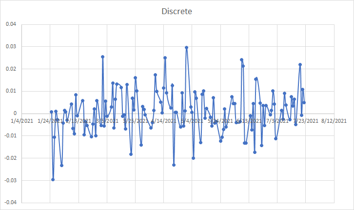
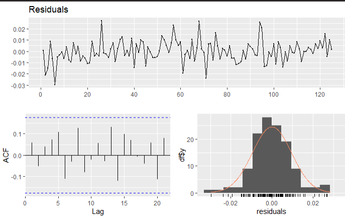
Upon plotting each column prepared in the preprocessing stage, we see that returns are enmeshing the zero-mark moving up and down through the entire timeframe of analysis. An image of this is shown below and gives quite some insight. Cumulatively this shows that a hypothesis that the average of differencing the stock returns can be a number zero or close to it. However, this is not key. What is, is that this is the volatility structure of the security or index. The returns movement away from the mean both up and down show the volatility of the security. An average of this movement can thus be considered the volatility factor. This is the variance of the log returns.
Finding the volatility of a security through this method is known as using the Market Model. The averages of returns are the average daily return of the security or index during that period, while the variation shows the volatility of the security. The market model uses the dynamics of supply and demand to try and predict the price and quantity of sold stocks. The question after this phase is whether is this the best method to predict, stock volatility. This method is not only deterministic it is also not in line with other market conditions.
- Capital Assets Pricing Model
The other method and most commonly used to predict stock volatility is the Capital Assets Pricing Model. The methodology is used mostly to calculate systematic risk and the expected return of the asset. CAPM is especially good for pricing very risky assets. Systematic risk are factors posed externally to the stock. Thus, they are all common to the entire market. This might include, pandemics such as in the case of 2020, economic recessions, government policies and so on. These risks are undiversifiable and, in most cases, cannot be prevented. CAPM adds to the market model something very crucial. Investors expect returns based on the volatility shakes they experienced and the time value for money, as such CAPM uses the risk-free rate to show the time value for money and uses a metric known as beta to show the volatility experienced by the security.
- Levy-Alpha Stable Volatility
Understanding this factor is just the tip of the analysis. Commonly when pricing options the volatility factor is derived from the two models addressed in the previous sections. However, our goal is to price options using volatility generated from the Levy-alpha stable distribution. A number of assumptions must be made to critically evaluate this process and lay down a strong foundation to the experimentation segment of the analysis. There is a lot of controversy when the prospect of estimating risk and volatility is affiliated to distributions with unbounded variations are used and many economists and financial experts defend the normal law which is the one used today. However, a lot of study has shown better description of the true nature of stocks and shocks through stable distributions. What these models try to calculate is the probability of the risk of fluctuations and thus in all aspects such a fit would be impeccable. Reading the block quote below from the Political Calculator, 2019, gives a better look into the subject matter. (The blockquote can be removed if not necessary in the proofing procedure)
If the volatility of stock prices followed a normal Gaussian distribution, we would expect that:
- 3% of all observations would fall within one standard deviation of the mean trend line
- 5% of all observations would fall within two standard deviations of the mean trend line
- 7% of all observations would fall within three standard deviations of the mean trend line
But that’s not what we see with the S&P 500’s data, is it? For our 17,543 daily observations, we instead find:
- 7% of all observations fall within one standard deviation of the mean trend line
- 3% of all observations fall within two standard deviations of the mean trend line
- 6% of all observations fall within three standard deviations of the mean trend line
Already, you can see that the day-to-day variation in stock prices isn’t normal, or rather, is not well described by normal Gaussian distribution. While there are about as many observations between two and three standard deviations of the mean as we would expect in that scenario, there are way more observations within just one standard deviation of the mean than we would ever expect if stock prices were really normally distributed.
Additional discrepancies also show up the farther away from the mean you get. There are more outsized changes than if a normal distribution applied, which is to say that the real world distribution of stock price volatility has fatter tails than would be expected in such a Gaussian distribution.
When a Levy distribution is fitted in four more index options that is S&P 500, Nikkei 225, Dow 30 and SSEC with large enough sample sizes, it shows even more robust results. Not only does it explain the phenomena extremely well, it fits the model with near accuracy. For all indexes the levy outshines the Gaussian in describing the variation of stock prices. Thus in terms of the GCLT (General Central Limit Theorem), Levy alpha is way more suitable at fitting the log returns of the security compared to the gaussian. The alpha stability parameter across all analysis shows a movement towards the 1.6 upon increase of data points and converges at this point except in rare cases such as the recessions. This value is definitely lower than the alpha value of the gaussian which is 2. The beta value which normally is a negative shows skewness in the stock or the index under sample. Thus, even though both methodologies do not fully expose the concentration of the log returns towards the center the Levy-alpha comes much closer to this in comparison to the Gaussian. Having this layout, there is now a clear roadmap to the investigation to be done. There is need to fit the stock prices of Pfizer and the Dow Index with the Levy-alpha stable distribution to find the concentration parameters of the distribution that is alpha (), the shape parameter, and beta(), the rate parameter. This model will better explain the volatility which can then be used in the pricing of the options. Having unambiguity in the lifecycle of an analysis is the most critical event of success and will lead clearly to the goal at hand.
- Experimentation and Results
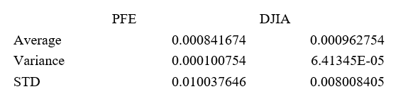
This section is the implementation of the concepts raised in previous sections. The first is calculation of the market model. This is relatively easy to do as it requires a descriptive statistics approach to the log returns of the security and the index. Through the market model, the daily returns and the daily volatility is estimated. The daily returns throughout the entire period is the average of the returns which is calculated using the mean () function in the R package,. The next parameter to calculate is the standard deviation which is the volatility. The values are then annualized to find the yearly return and volatility of the stock. The annualization is almost similar to compound annual growth return (CAGR) which is found by dividing the daily return by the square root of the time of growth. The R implementation is found in the codex. The other important statistic to derive is the risk-free asset return. It is also evaluated in the same methodology by finding the average of the risk-free asset column. In this project, implementation of the market model is done via both R and Excel. Since both are good data analysis frameworks, having a combination of both views reduces the chances of finding the wrong value for an answer. The tables and results are shown below.
Implementation of the CAPM model is next. The key principle to understand is that this model wants to predict the systematic risk, this is basically risk across the entire market. Or the effect the market to the stock. Thus, finding undiversified risk. Thus to find the effect on the market to the security price, linear regression is used. The dependent variable is the PFE stock returns while the independent variable is the DJIA index returns. The coefficient arising from this analysis is the beta coefficient which is the systematic risk of the security. The regression is implemented using the lm() function in R.
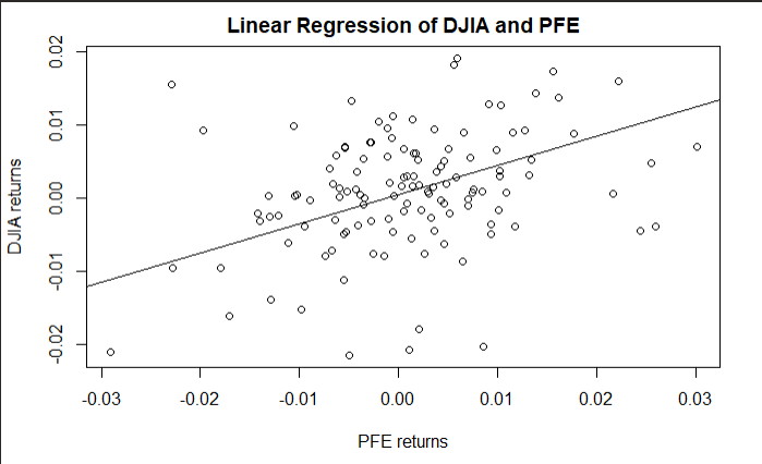
The fit is then plotted for even more clarity. The intercept in this scenario is the Jensen Alpha which is also an important coeffient in estimating the ROA. However, since what is needed in this scope is the volatility coefficient the beta works perfectly. The implementation is also done in Excel using the regression function in the data analysis module. The results are the same. To confirm that the beta is actually true, the t-stat and the p-value are measured.
The following table shows the results on the linear regression. This is done using the stargazer library which returns a lLaTex table of results for professional formatting. The t-value and p-value being within range of the alpha value show that the return is actually correct and that the beta is 0.39.

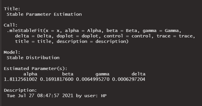
The final implementation is finding the Levy Alpha distribution of the return data of both the index and the stock. The implementation of this is a lot of mathematical implementations but since we are use a statistical language, the module for this particular heavy lifting has already been created. Thus, with just a few modifications, the concerned values are predictable. The goal is to find the best concentration parameters to describe the dataset. The choice of initial alpha and beta values will affect greatly the time it takes for the algorithm to run. The algorithm is also very critical and for each integration it works it raises a concern if it does not have a convergence property. When the limit approaches infinity the algorithm crashes and thus maximum precision and clarity is needed for proper implementation. Since from our previous literary analysis, we understood that most alpha values for most stock indexes approach a 1.6 value and the gaussian is 2.0. A median value between the two would be a good place to start to allow the model run to either of the sides. Since our data values are also less, there is a likelihood it will not achieve the 1.6 mark and thus we try to be close as much as possible to ensure minimal running of the algorithm. Thus, even though , there is great likelihood, the alpha value is between the mark. Thus, a compromise value of 1.75 is chosen as the starting value.
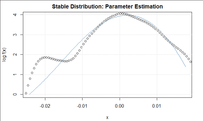
Figure 1.1 Dow Jones Levy Alpha Distribution
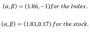
The initial beta value is also chosen in the same fashion. Since in most previous analysis, most beta values ranged in the negative domain, this would be a good place to start. In any case, . However, since we have a feeling that even though the Gaussian does not completely describe the variations it comes close with a beta of around 0.5. However, analysis has that beta was around the -0.16 mark. Thus, to reduce running time of the algorithm as much as possible which is done by making an estimation beta ranges , even though it can be higher or lower than this, this is the optimal choice for the algorithm and thus a beta value compromise of 0 is chosen. This reduces the running and logging time as much as possible. The model is then allowed to run and the following results are estimated. The alpha value is 1.811 as expected by the assumptions and the beta value is 0.17 also within the range of estimation. This is repeated for the index and the alpha value of 1.86 and beta value of -0.99 are estimated. This is practically:
Thus, having estimated the Levy alpha distribution for the data the new volatility can be estimated.
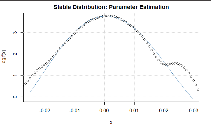
Figure 1.1 Pfizer Levy-Alpha Distribution
Option Pricing
Black Scholes Model using CAPM and Market Model Volatility
A lot of economists and financial analysts call and argue that the Black Scholes model is one of the most beautiful and robust formula invented in the discipline. It is so robust that it incorporates so many aspects surrounding an option that its prediction is near accuracy. However the sigma factor it uses is volatility calculated by other models surrounding the security. It is an ordinary differential in the form of a separable equation that utilizes five key inputs: stock price, interest rates, the time of expiration of the option, the volatility or risk surrounding it and the strike or exercise price. Options are derivatives or as most people call them, “stock insurance.” The key principles to note is that the higher the volatility the higher the price of the option. The longer the time to expiration the higher the price of the option and finally the underlying stock price also affects the price of the option. However, for our model implementation the most important variable is the volatility factor. It also incorporates the use of the risk-free asset for its estimation regarding the time value for money (TVM).
The qrmtools package found along other R distribution shall be used for the analysis. The annualized volatility from the market model shall be used
The QRM package shall be used for most of the heavy lifting in this phase. It shall be used for the Black Scholes model. It will also be used to measure the Greeks. What is needed is to run the function a number of times with the desired parameters as estimated in previous section. The stock price at time of purchase is used as initial while the sigma or volatility is chosen from the annual risk calculated by the market model. The risk-free rate which was estimated as 0.09 is also added and the time to expiration which is 6 months is incorporated in the calculations. The strike price will be a range all in the money. This means that with a gap of 2, the first strike price to be estimated will be 2 points lower than the stock price. That will be 44 less 2 being 42. Each will have an interval of 2 and thus 40, 38, 36 and so on. This can be repeated using the Beta from the CAPM though not necessary. The description in previous sections was to show the possible ways of achieving the desired target. The resulting European call option prices are stored in a table that will be used for comparison with the once generated from the Levy Alpha. The next phase will involve using the beta coefficient generated from the fitted stable distribution as the volatility factor in the Black Scholes and the resulting values will also be stored in a table for computation. Another key metric that will later on be calculated is the implied volatility. This metric will be tackled in the next section together with the alpha implementation.
Fourier Transform using Stable Distribution
This is the culmination of the entire research paper. This method is not one of its kind but it is among the few that have been constructed. Little is known about usage of the Fourier in the calculation of options as the method takes a toll on the computation machine under use. It involves a number of constrains as it is based heavily on integration unlike the Black Scholes. The functions under study are also very robust and heavy and thus generating an answer requires time and computation power. The effect to the machine was so severe that it overheated while running. To generate call options however via this method requires patience and wide knowledge on functional implementation and passing arguments to a function. The section was done using python as it works best with the arrays and matrices generated while computing. It also has a wide library support geared towards scientific and mathematical domains. These include SciPy, NumPy. Matplotlib and Pandas.
The next step is defining the characteristic function under investigation. However in our model this is not done explicitly as the a very good implementation of this was done in a previous paper by Carr & Muddan, 1999. The following code shows the characteristic function which is similar to Levy Alpha defined in this previous paper. The characteristic function takes all the necessary inputs as it will be used in the next section. The python implementation of this is heavily noted to make good guidance to the party following the code. The next step is passing the characteristic function through the inverse of the Fourier transform. This will be known as the fast Fourier transform. This is done with the values to be tested that is the strike price, the asset price, the time to expiration, the alpha of the model, the volatility which is the alpha of the described model and finally the starting time.
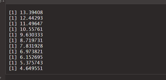
Together this function will run to create a matrix of complex numbers which shall be solved using the Simpson’s rule. The rule is used for integration as the values are present. Other metrics have been added to the model to ensure it does not wander of to infinity. The following snippet is the code implementation of the fast fourier transform and the Simpson’s rule. The implementation is wrong but follows the same procedure as the first two chapters and thus a description would a repeat of the same. The resulting predictions are then stored as shown below.
Conclusion
Creating a feasible and viable portfolio that will yield results competitive to the market is no straightforward task-it requires the incorporation of many methodologies discovered all through financial history. Past data is as critical as the future, yet it does not always reflect on what will happen. Like any game of bets, one might win or lose. Thus, minimizing risk through diversification and proper portfolio determination to maximize and optimize yields makes up a good and solid investment structure.
References
Kanellopoulou, S., & Panas, E. (2008). Empirical distributions of stock returns: Paris stock market, 1980–2003. Applied Financial Economics, 18(16), 1289-1302.
https://edoc.hu-berlin.de/bitstream/handle/18452/4526/8.pdf
Kogon, S. M., & Manolakis, D. G. (1996). Signal modeling with self-similar/spl alpha/-stable processes: the fractional Levy stable motion model. IEEE transactions on signal
processing, 44(4), 1006-1010.
https://ieeexplore.ieee.org/abstract/document/492557/
Kogon, S. M., & Williams, D. B. (1998). Characteristic function based estimation of stable distribution parameters. A practical guide to heavy tails: statistical techniques and
applications, 311-338.
Nolan, J. P. (2001). Maximum likelihood estimation and diagnostics for stable distributions. In Lévy processes (pp. 379-400). Birkhäuser, Boston, MA.
https://link.springer.com/chapter/10.1007/978-1-4612-0197-7_17
Rimmer, R. H., & Nolan, J. P. (2005). Stable distributions in mathematica. Mathematica Journal, 9(4), 776-789.
/links/542950e20cf2e4ce940c9dc6/Stable-Distributions-in-Mathematica-Robert-H-Rimmer.pdf
Scalas, E., & Kim, K. (2006). The art of fitting financial time series with Levy stable distributions. arXiv preprint physics/0608224.
https://arxiv.org/pdf/physics/0608224
Appendix
def mertonCF(u, x0, T, r, sigma, lmbda, mu, delta):
omega = x0 / T + r – 0.5 * sigma ** 2 \
– lmbda * (np.exp(mu + 0.5 * delta ** 2) – 1)
value = np.exp((1j * u * omega – 0.5 * u ** 2 * sigma ** 2 +
lmbda * (np.exp(1j * u * mu –
u ** 2 * delta ** 2 * 0.5) – 1)) * T)
return value
# from here one could use the Lewis (2001) approach with numerical integration
# or as we will do, follow th Carr-Madan (1999) Approach and use FFT
# Carr-Madan Approach with FFT
def fft_call(S0, K, T, r, sigma, lmbda, mu, delta):
k = math.log(K / S0)
x0 = math.log(S0/S0)
g = 4 # factor to increase accuracy
N = g * 2048
eps = (g * 150.0) ** -1
eta = 2 * math.pi / (N * eps)
b = 0.5 * N * eps – k
u = np.arange(1, N + 1, 1)
vj = eta * (u – 1)
# Modificatons to Ensure Integrability
if S0 >= k: # ITM case
alpha = 1.5
v = vj – (alpha + 1) * 1j
modCF = math.exp(-r * T) * mertonCF(
v, x0, T, r, sigma, lmbda, mu, delta) / (alpha ** 2 + alpha – vj ** 2 +
1j * (2 * alpha + 1) * vj)
else: # OTM case – this has 2 modified characteristic functions since is can be dampened twice due to its symmetry,
# these are weighted later on
alpha = 1.1
v = (vj – 1j * alpha) – 1j
modCF1 = math.exp(-r * T) * (1 / (1 + 1j * (vj – 1j * alpha))
– math.exp(r * T) /(1j * (vj – 1j * alpha))-
mertonCF(v, x0, T, r, sigma, lmbda, mu, delta) /
((vj – 1j * alpha) ** 2 – 1j * (vj – 1j * alpha)))
v = (vj + 1j * alpha) – 1j
modCF2 = math.exp(-r * T) * (1 / (1 + 1j * (vj + 1j * alpha)) –
math.exp(r * T) /(1j * (vj + 1j * alpha))-
mertonCF(v, x0, T, r, sigma, lmbda, mu, delta) /
((vj + 1j * alpha) ** 2 – 1j * (vj + 1j * alpha)))
# Fast Fourier Transform
kron_delta = np.zeros(N, dtype=np.float) # the Kronecker Delta Function is 0 for n = 1 to N
kron_delta[0] = 1 # function takes value 1 for n = 0
j = np.arange(1, N + 1, 1)
# Simpsons Rule
simpson = (3 + (-1) ** j – kron_delta) / 3
if S0 >= 0.95 * K:
fftfunction = np.exp(1j * b * vj) * modCF * eta * simpson
payoff = (fft(fftfunction)).real # calls numpy’s fft functions
call_value_pre = np.exp(-alpha * k) / math.pi * payoff
else:
fftfunction = (np.exp(1j * b * vj) * (modCF1 – modCF2) *
0.5 * eta * simpson)
payoff = (fft(fftfunction)).real
call_value_pre = payoff / (np.sinh(alpha * k) * math.pi)
pos = int((k + b) / eps) # position
call_value = call_value_pre[pos]
return call_value * S0
#print(fft_call(S0, K, T, r, sigma, lmbda, mu, delta))
str = range(32,40,0.5)
for i in str:
print(fft_call(S0, i, T, r, sigma, lmbda, mu, delta))