DETERMINANTS OF AUDITING FEES AMONG UK FIRMS

1- Introduction

The study aims to investigate empirically the relationship between auditing fees as a dependent variable and five independent variables, namely: turnover, profit, total assets, number of employees and type of auditor. This study belongs to a stream of accounting research that investigates the determinants of auditing fees.

The sample consisted of private companies that met the following conditions:

• Fewer than 50 employees.
• Turnover less than £5.6 million.
• Total assets less than £2.8 million.
• Located only in Wales and London.
• The primary sector codes are 15 (manufacturing of food and beverages) and 55 (hotels and restaurants).

This yielded a sample of 122 companies during the period under investigation.

The study aims to:

• Investigate the differences in turnover, profit, total assets, number of employees and auditing fees between companies that use one of the Big 4 to audit their financial statements and companies that use a non-Big 4 auditor.
• Build a model to explain the relationship between the dependent variable (auditing fees) and the independent variables (turnover, profit, total assets, employee numbers and auditor type). This model will be helpful for prediction purposes.

2- The Dependent and Independent Variables

2-1- Dependent Variable

The dependent variable reflects the fees the company paid for the auditing of its financial reports.

• Independent Variables

The independent variables are:

• Company turnover: the number of sales during the period under examination.
• Company profit (loss): the profit (loss) of a company at balance sheet date.
• Company total assets: the total assets at balance sheet date.
• Employee numbers: the number of the employees during the period under investigation.
• Auditor type: whether the auditor is one of the Big 4 or a non-Big 4 auditor. The Big 4 auditors are: KPMG, PricewaterhouseCoopers, Deloitte Touché Tohmatsu and Ernst & Young.

3- Data Analysis

The researcher employed the following statistical tools and tests:

• Descriptive statistics
• Mann-Whitney test
• Correlation
• Regression

These statistical tools and tests will each be discussed in the following sections.

3-1-Descriptive statistics

This section provides basic descriptive statistics about the variables under investigation. For each variable, the researcher divided the data according auditor type (Big 4 and non-Big 4). The aim of exploring the data was to identify whether the data was normally distributed since this would have an impact on the choice of the most suitable test. In general terms, there are two main statistical tests, namely parametric and non-parametric tests. The basic assumptions for parametric tests are (Field 2002):

1- Data is normally distributed

2- Constant variance (homogeneity of variance)

3- Interval data where the distance between points in a scale is equal

4- The observations from different objects are independent

Consequently, any violation for these assumptions would mean that the researcher must employ a non-parametric test. Non-parametric tests have some advantages (Siegel and Castellan 1988):

• They hold few assumptions regarding the data.
• Compared with parametric tests, their interpretation is more direct.
• They are suitable for cases where the sample size is relatively small.

The basic statistics for the dependent and independents variables are discussed below.

A-Turnover

The mean and the standard deviation of turnover for companies that are audited by one of the non-Big 4 are 2587.8 and 1435.7 million respectively. The data is positively skewed (0.502) and the kurtosis is -0.694. For companies that are audited by one of the Big 4, the mean and the standard deviation are 2827.12 and 1242.4 million respectively. The data is positively skewed (0.546) and the kurtosis is -1.004.

B- Profit

For companies that are audited by one of the non-Big 4, the mean and the standard deviation are 89.54 and 1131 million respectively. The data is positively skewed (1.01) and the kurtosis is 28.96. The mean and the standard deviation for companies that are audited by one of the Big 4 are 29.29 and 411.02 million respectively. The data is negatively skewed (-0.815) and the kurtosis is 1.821.

C-Total Assets

The mean and the standard deviation of total assets for companies that are audited by one of the non-Big 4 are 1459.65 and 810 million respectively. The data is negatively skewed (-0.154) and the kurtosis is -1.262. For companies that are audited by one of the Big 4, the mean and the standard deviation are 1544.58 and 769.5 million respectively. The data is negatively skewed (-0.211) and the kurtosis is -1.007.

D- Employee Numbers

The mean and the standard deviation of employee numbers for companies that are audited by one of the non-Big 4 are 42 and 27 employees respectively. The data is positively skewed (0.414) and the kurtosis is -0.791. For companies that are audited by one of the Big 4, the mean and the standard deviation are 43 and 26 employees respectively. The data is positively skewed (0.214) and the kurtosis is -1.039.

E-Auditing Fees

For companies that are audited by one of the non-Big 4, the mean and the standard deviation of auditing fees are 9.05 and 7.35 thousand respectively. The data is positively skewed (3.13) and the kurtosis is 14.54. For companies that are audited by one of the Big 4, the mean and the standard deviation are 7.376 and 5.03 thousand respectively. The data is positively skewed (0.894) and the kurtosis is 0.586.

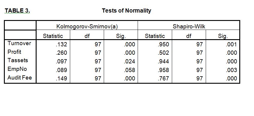
These descriptive results, which are supported by a histogram, stem-and-leaf, normal Q-Q plots and a box plot, indicate that the data is not normally distributed. In order to test whether this deviation from the normal distribution is significant or not, the researcher applied Kolomogorov-Smirnov and Shaoiro-Wilk tests. The results of these tests indicated that the turnover and auditing-fee data for both non-Big 4 and Big 4 companies were not normally distributed (p<0.05).

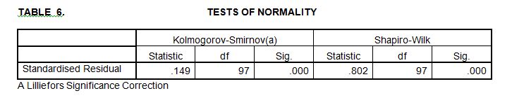
With regard to profit, total assets and employee numbers, the data of the non-Big 4 is not normally distributed (p< 0.05) while the data of the Big 4 is normally distributed (p> 0.05). The following table summarises these results:

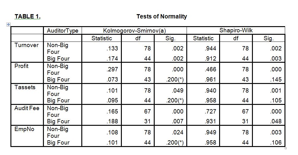
These results support the use of non-parametric tests to investigate the differences between the companies that use one of the Big 4 auditors to audit their financial statements and those that use one of the non-Big 4 auditors in terms of turnover, profit, total assets and employee numbers. The results further support the use of the Mann-Whitney test and Spearman’s rho to examine the correlation between the variables.

3-2-Mann-Whitney

The Mann-Whitney test is a non-parametric test used to test differences between the mean ranks of two groups. The hypotheses to be tested are:

H₀: There are no significant differences in turnover, profit, total assets and employee numbers between companies that use one of the Big 4 to audit their financial statements and companies that use one of the non-Big 4 auditors.

H₁: There are differences in turnover, profit, total assets and employee numbers between companies that use one of the Big 4 to audit their financial statements and companies that use one of non-Big 4 auditors.

Table 2 summarise the results of the test.

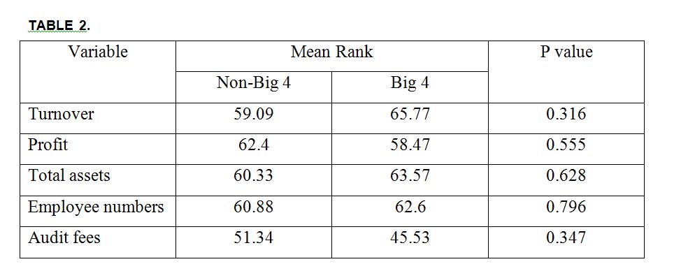
The results of the Mann-Whitney test indicate that the null hypothesis cannot be rejected (p>0.05). Therefore, there are no significant differences in turnover, profit, total assets and employee numbers between companies that use one of the Big 4 to audit their financial statements and companies that use one of the non-Big 4 auditors.

3-3-Correlation Matrix

A Spearman’s rho was used because the descriptive statistics indicated that the variables were not normally distributed.

The matrix below summarises the correlation between the variables.

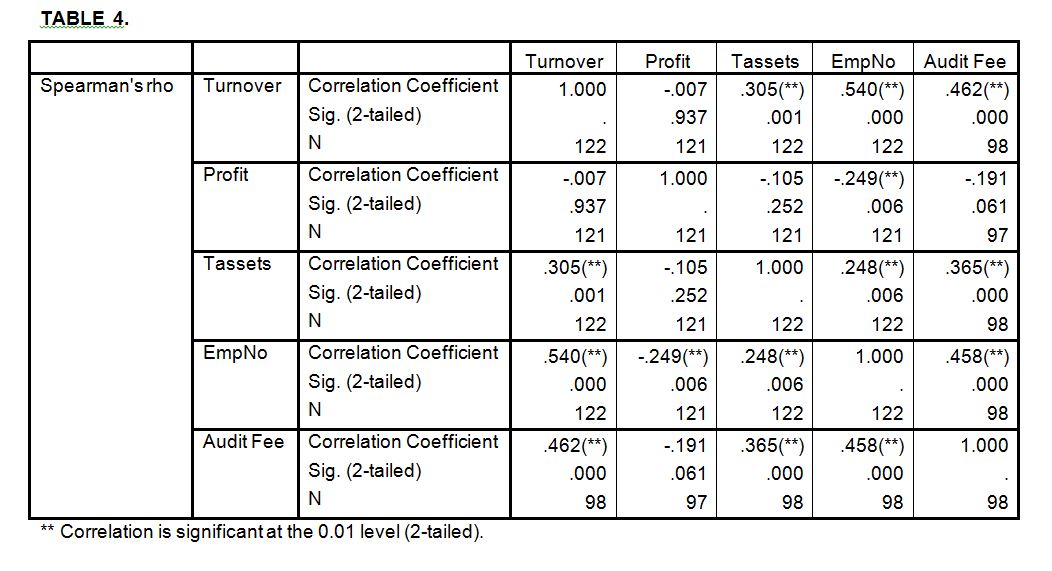
The results of the correlation matrix indicate that:

• There is a significant positive relationship between audit fees, turnover (0.462), total assets (0.365) and employee numbers (0.458) at a significance level of 1%. There is a negative association between auditors’ fees and profit (-0.191) but this relationship is not significant at a significance level of 5%.
• There is a significant positive relationship between employee numbers, turnover (0.54) and total assets (0.248) at a significance level of 1%. There is a negative association between employee numbers and profit (-0.249) but this relationship is significant at a significance level of 1%.
• There is a significant positive association between total assets and turnover (0.305) at a significance level of 1%. There is a negative association between total assets and profit (-0.105) but this relationship is not significant at a significance level of 5%.
• There is a negative association between profit and turnover (-0.007) but this association is not significant at a significance level of 5%.

3-4- Regression

A- Regression Model

In this section, the researcher attempts to obtain a regression model that can predict the auditing fees (dependent variable) for a sample comprising private companies located in London and Wales. The researcher specified the following as independent variables: turnover, profit, total assets, employee numbers and auditor type. The regression model can be expressed as follows:

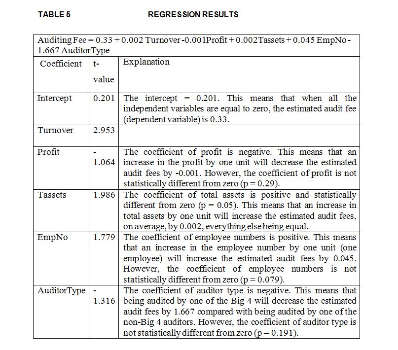
Auditing Fee = a + b₁Turnover + b₂ Profit + b₃Tassets + b₄EmpNo + b₅AuditorType + e

where:

a = regression intercept.

Auditing Fee = fees that the company paid for auditing its financial reports.

Turnover = company sales during the period under examination.

Profit = company profit (loss) at balance sheet date.

Tassets = the total assets at balance sheet date.

EmpNo = number of company employees during the period under investigation.

AuditorType = dummy variable (0= non-Big 4 auditor, 1=Big 4 auditor).

e = error term.

B- Regression Model Results

The results indicate that the adjusted R² for the model equal 27.1%, F _{(5, 91)} = 8.122, p < 0.001. Therefore, the model is statistically significant overall. In other words, the independent variables significantly explain 27.1% of the variations in the dependent variable (auditing fees). Other variables that were not included in the model could explain 72.9% of the variation in the dependent variable. The regression results are summarised in Table 5.

C- Testing the Assumptions of Regression Analysis

1. Normality Assumption

Many statistical tools can be used to detect violations of normality assumptions. For example, a normal Q-Q plot, box plot, histogram and steam and leaf for standardized residuals can be used to check the normality assumption. A review of these statistical tools indicated that the distribution of the residuals was not normal: the positive skew of standardized residuals is 2.675 while kurtosis is 14.08. To check whether this violation of normality assumption was significant, the researcher used two statistical tests. The Kolmogorov-Smirnov and Shapiro-Wilk tests were significant (p < 0.001). Therefore, the null hypothesis that the distribution is normal is rejected. This means that the residual is not normally distributed.

It could be concluded that the violation of the normality assumption could have a severe impact on the results. Lewis-Beck (1993) stated that ‘the normality assumption, for instance, can be ignored when the sample size is large enough, for then the central limit theorem can be invoked’ (Lewis-Beck 1993, p. 22). Kvanli et al. (1996) point out that the violation of normality assumption occurs when the distribution of the residuals is extremely skewed. However, the sample under investigation is small (n = 97) and the distribution of standardized residual is considerably positively skewed (2.675). Therefore caution should be exercised in interpreting the results.

1. Linearity

In order to check the linearity assumption, the researcher used a scatter-plot of the standardized predicted value and the standardized error. The scatter plot does not indicate a curved line and therefore it can be concluded that there is no violation for the linearity assumption.

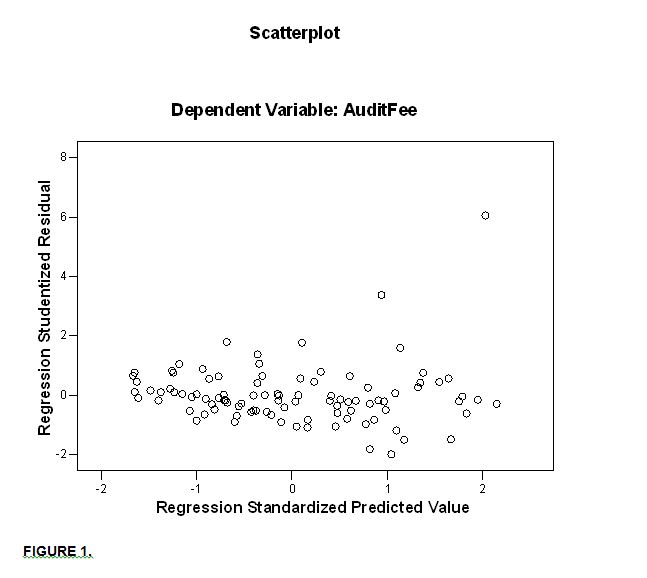
• Homoscedasticity

A scatter plot of the standardized predicted value and the standardized error indicates that there is a dispersed random array of dots. Therefore it can be concluded that there is no chance of violating the homoscedasticity assumption.

1. Independence errors

To examine whether the residuals are correlated, the Durbin-Watson test was used. The test statistics can vary between 4 and 0; a value of 2 indicates that the residuals are not correlated. Therefore, a test value which is greater than 3 and less than 4 is considered to be cause for concern (Field 2002). The Durbin-Watson value is 1.935, indicating that the residuals are uncorrelated.

1. Multicolinearity

Many measures can be used to detect multicolinearity between independent variables. The researcher used a correlation matrix of independent variables and the variance inflation factor (VIF) to identify the existence of multicolinearity. The correlation matrix and VIF indicated that multicolinearity would not be a problem. As rule of thumb, multicolinearity may appear when the correlation between independent variables is high: for instance, 0.8 or above (Field 2002). The highest correlation was 0.52 between turnover and employee numbers. As a rule of thumb, the VIF should be less than ten (Kvanli et al. 1996). An examination of the VIF showed that all independent variables had a VIF of less than ten (the maximum VIF was 1.556 for turnover).

1. Outliers and Influential Points

Outliers and influential points are cases that differ significantly from the general trend. Outliers and influential points produce a biased regression model and can have a severe impact on the results because they influence the estimated coefficients (Anderson et al. 2007). There are many ways to detect outliers and influential points. One of these is the standardized residual: it is expected that 95% of cases have a standardized residual within ± two. The sample under investigation consists of 97 observations; therefore it is reasonable to expect that about five cases (97 * 5%) would have a standardized residual outside ± two. Casewise diagnostics indicate that only two cases (case 11 and 43) exceed the limits. Therefore it can be concluded that the existence of outliers would not have a severe impact on the results.

In order to detect the influential points, the leverage and the Cook distance could be used. Leverage estimates the influence of the observed value of the dependent variable over the predicted values (Kahane 2001). The researcher used 3(K+1)/n as a cut-off point to determine observations that have excessive influence (Anderson et al. 2007). The cut-off point ([3(5+1)]/97) is 0.185. Casewise diagnostics indicate that the maximum leverage value is 0.527. Examining the leverage of all the observations revealed that only two observations exceeded the limit, namely observation 53 (leverage is 0.527) and observation 78 (leverage is 0.36).

Cook’s distance is a measure of the overall influence of a case on the model. It is recommended that values > 1 could be considered as a cause of concern (Field 2002). Casewise diagnostics indicate that the maximum Cook’s distance value is 0.356: this means that no observation exceeded the limit. Therefore it can be concluded that the outliers and influential points have no great impact on the results.

• Study Limitations and Future Research

The study has several limitations which should be taken into consideration when interpreting the results. The first limitation is the sample size used in the study. Of course, if a large sample had been used, the results may have been supported. The second limitation is that only private companies located in Wales and London were used. Moreover, the sample consisted of only two primary sector concerns – manufacturing of food and beverages and hotels and restaurants. In the long term, these drawbacks will limit possible statistical generalisations that could be made from this study.

Recommendations for future research include using a large sample. The results indicate that 72.9% of the variation in the dependent variable was explained by independent variables that were not included in the study. Therefore, future research could investigate the impact of other independent variables such as companies from different geographical locations and economic sectors in the UK. Including variables such as the gearing and liquidity ratios or including public companies may enhance the predictability power of the regression model.

• Bibliography

– Anderson, D. R., Sweeney, D. J., Williams, T. A., Freeman, J. and Shoesmith, E. 2007. Statistics for Business and Economics. London: Thomson Learning.

Field, A. 2002. Discovering Statistics using SPPS for Windows. London: Sage Publications.

– Hair, J. F., Anderson, R. E., Tatham, r. L. and Black W. C. 1995. Multivariate Data Analysis: with readings. Englewood Cliffs, N.J: Prentice Hall.

– Kahane, Leo H. 2001. Regression Basics. Thousand Oaks: Sage Publications,

– Kvanli, A. H., Guynes, C. S. and Pavur, R. J. 1996. Introduction to Business Statistics: A Computer Integrated Data Analysis Approach. 4ed. New York: West Publishing Company.

– Lewis-Beck, M. S. 1993. Applied Regression: An Introduction. In: Lewis-Beck, M. S. ed. Regression Analysis. New York: Sage Publications. pp. 1-68.

– Siegel, S. and Castellan, N. J. 1988. Nonparametric statistics for the behavioral sciences 2^nd ed. New York: McGraw-Hill.